Know your loop before you attempt to tune your loop, part 2

In the last article for this topic, we discussed the importance of field data collection and the importance of a methodical approach to proportional-integral-derivative (PID) tuning. I introduced the concept of the bump test and that its results would help guide the steps and equations used in proper tuning. Here, I will explore that concept in greater detail. At ECS, we use a visual tool for data collection in every instance. The tool may be part of a controller suite, or it may be standalone but, in any case, it is imperative to capture accurate information about the performance of your system before planning and then programming a solution.

This article will focus on tuning concepts for self-regulating loops as they make up the majority of applications in the industrial field. A common example of this type of loop is a flow control which varies flow through a pipe via either variable speed control on a pump or a position-controlled valve. In this example, the flow can be adjusted by speed adjustment of the pump or position of a valve and the result of the change ordered from the controller is stable and is generally fast and repeatable.

Courtesy: ECS Solutions

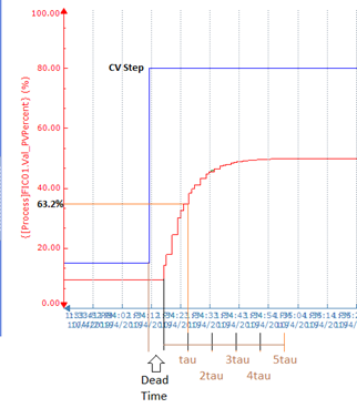
First, I place the system in manual mode and establish a visual graph which shows the process variable (Pv) and control variable (Cv).  I take care to observe both items as a percentage of their overall capability, not in either or both engineering units. Once I can see these elements and I understand their safe operating limits, I define an initial Cv and wait for the Pv to stabilize. If the system stabilizes then it is confirmed that I have a self-regulating loop. Next, I note an initial time, T1, and I modify the control variable with a large step. I measure the time between my modification and when the process variable begins to respond or T2 and the difference between these defines the dead time of my system. An ideal theoretical dead time would be zero, but this is not possible. If the deadtime is too large, then there is likely a physical problem with the system, and it is unlikely we will achieve satisfactory results with programming changes only.

I observe how the disturbance I introduce affects the output, specifically establishing a ratio between the Cv disturbance and Pv response (Process Gain). A 1:1 reaction as measured in percentage by to my disturbance would be ideal but anything that reacts within the range of 0.5to 2 is acceptable. If the Process Gain is smaller than 0.5 the process it undersized and when exceed 2 the process is oversized. It is possible to re-scale the Pv if it isn’t in the desirable range but this should not be used as a substitute to proper resolution and also not to mask physical problems. It should be noted that most sensors will perform linearly, however; there are situations where a non-linear sensor is required and it may be necessary to linearize an output within the sensor itself, a conditioner, or via code within the system controller. This is a detailed discussion which is too exhaustive to cover in this article.

Continuing to watch the system response, I measure the time it takes to achieve a change to 63.25% in our Pv and this is noted as 1 Tau, which is used to establish the system gain. Finally, I observe the Pv’s response curve, noting in general that the response drives up (or down) towards the Cv setpoint and settles out. This response is our stabilization time, and it will be the primary focus of our tuning later. I like to collect and note this baseline information multiple times at this phase at varying percentages of Cv to ensure that the system is repeatable at various points.

Armed with this information, I can now select the proper equation(s) to use for my tuning plan. The mathematical equations vary slightly between independent and dependent gain but, in either case, you have the variables that you need. Your initial work should be by hand and then later applied to the controller logic. Using Lambda tuning formulas you can compute derivative, integral, and gain. These are your starting points for adjustments within the controller instructions.  It should be noted that controller logic varies a bit from brand to brand and even potentially model to model but the required input information is still there.

In future installments of this series, I will detail specific Lambda formulas and the corresponding logic from one brand of controller so that readers can see the theory, generated constants, and the resulting code.

Do you have experience and expertise with the topics mentioned in this content? You should consider contributing to our WTWH Media editorial team and getting the recognition you and your company deserve. Click here to start this process.