Whenever a new control system is proposed for an automated plant, a manager, engineer, or operator invariably asks how the system will react to certain events or conditions in the plant. What happens when the ambient temperature drops below freezing? What will the control system do if the conveyor suddenly stops? Will the robot arm be able to squeeze through that opening with a part in it...
KEY WORDS
Process control & instrumentation
Simulation
Modeling
Testing
System analysis or design
Sidebars: SIMULATION TERMS
Whenever a new control system is proposed for an automated plant, a manager, engineer, or operator invariably asks how the system will react to certain events or conditions in the plant. What happens when the ambient temperature drops below freezing? What will the control system do if the conveyor suddenly stops? Will the robot arm be able to squeeze through that opening with a part in its grip? These can literally be million dollar questions since a control system can either run the plant more profitably or make matters worse when unexpected situations occur.
Unfortunately, it is not always obvious from the design of a proposed control system whether it will be able to do more good than harm. A continuous process controller may be able to handle setpoint changes smoothly, yet fluctuate wildly when a load disturbs the process variable. A fleet of automatic guided vehicles may be able to deliver parts to the assembly line for months without mishap, then fail catastrophically when two of them happen to reach the same point at the same time.
The only certain way to test how a proposed control system will handle every conceivable situation is to design it, install it, and try it out. However, this can be a very costly means of uncovering design flaws. A control system failure can shut down the plant and require expensive modifications. In the worst case, the entire control system may have to be scrapped, redesigned, and rebuilt.
A better way
Testing a control system is much easier to do if the system is first designed in a computer-based virtual world. A simulated control system can be installed in a simulated plant without the expense of real equipment and without the risk of disrupting the real plant’s production. In this virtual world, both the plant and the control system exist only as customized code in some kind of a simulation computer or simulator .
Computer simulations allow all manner of extreme conditions and “what-if” scenarios to be tested safely If a test uncovers a flaw in how the control system handles a certain situation, the necessary modifications can be implemented and retested merely by updating the control system’s program in the simulator. Once all the what-if questions have been answered satisfactorily, the fully tested control program can be lifted right out of the simulator and run as-is in the real control system.
Simulations can be equally useful after the control system has been completely debugged and installed. As experienced operators run the real plant, new operators can be trained to do the same using a simulated plant and a simulated control system. Simulation training is often conducted in a mock-up of the control room equipped with all the operator displays used in the real thing. A simulator such as Trainer from Honeywell Hi-Spec Solutions (Phoenix, Ariz.) substitutes for the real plant and the real control system. However, if the simulation is realistic, the trainees don’t know the difference. They graduate ready to run the real plant themselves. This training regimen can be particularly effective in large, highly automated facilities where simulated “learning experiences” are much less costly than making real mistakes with the real plant.
Model the process
So how can all this be accomplished? Simulations can be implemented on virtually any computing platform using any number of commercial software packages. However, all simulations start with some sort of mathematical model that quantifies the behavior of the plant.
A typical plant model includes several equations with several variables that represent the inputs , the outputs , and the parameters of the plant. Anything that the control system does to influence the activities of the plant is an input. The measurable results of those control efforts are the outputs. The control system computes the inputs, which it needs to apply to the plant according to recent output measurements.
Conversely, the equations in the plant model show how the inputs affect the outputs, and the parameters dictate how much of an effect each input has on each output.
Just how the equations for a particular model should be structured and just what values should be assigned to each parameter are questions worthy of graduate study. Modeling can be a relatively simple matter if the behavior of the plant is obviously governed by natural laws such as physics, chemistry, or geometry (see the example in Figure 1). For more complex plants, however, empirical relationships based on statistical observations of the plant’s previous behavior may be required to produce a realistic model.
Once the plant model has been developed and tested for accuracy the rest is easy. The simulator takes an initial set of plant inputs and solves the model’s equations for the outputs that would result from the real plant. It then takes those outputs and uses the control program to compute the next set of inputs that would result from the real control system. The new inputs lead to new outputs which lead to new inputs ad infinitum. With each iteration, the new data are recorded and a simulated clock is incremented to represent the passage of time.
A simple simulation
Consider, for example, the teeter-totter shown in Figure 1. The position Y and velocity V y of the boy on the right are determined by the position X and velocity V x of the girl on the left as shown in equations [1] through [3]. Thus, the girl is the control system, the boy is the plant, and the board is the actuator that the control system uses to influence the plant.
Equations [1] through [3] constitute this plant’s model. The variables X and V x are the inputs, Y and V y are the outputs, and the dimensions a, b, and c are the parameters of the plant. A simulator would solve equations [1] through [3] for the values of Y and V y that correspond to the latest values of X and V x . The values of X and V x would in turn be calculated according to equation [4] which represents the control program.
The kinds of what-if scenarios that could be tested with this simple simulation might include the effects of varying the dimensions a, b, and c in the plant or the value of Y min in the control program. The steps in the control program could also be modified to test a more elaborate strategy for achieving the control system’s objectives.
Caveats
This teeter-totter simulation is a particularly simple example. Plant models for continuous processes generally involve several differential equations which need to be solved simultaneously. Even discrete manufacturing models that take the form of simple IF-THEN-ELSE equations can become considerably more complex when the plant is comprised of hundreds of devices with thousands of possible operating states.
Boundary conditions are another problem that can make a simulation more difficult. Physical constraints in the plant prevent the real inputs and outputs from exceeding certain upper and lower limits. In the teeter-totter example, the ground prevents both X and Y from assuming negative values. Consequently, their upper values are limited to c(1 + a/b) and c(1 + b/a), respectively. Extraneous values for both simulated variables might result if these boundary conditions are not incorporated into the plant model.
Worse still are the problems of unmodeled behavior . Any plant activity that is not somehow included in the plant model is a potential source of errors in the results predicted by the simulation. The plant model given by equations [1] through [3] does not account for the elasticity of the teeter-totter board, nor does it account for the inertia of either rider. The actual position of the boy will always lag the position predicted by the plant model. In this example, the errors resulting from the unmodeled behavior may not be significant. However, bridges and buildings have been known to collapse as a result of unexpected behavior that was overlooked in the simulation tests.
Even if all of the most significant plant behavior is incorporated into the model, a simulation can still give erroneous results if the model includes incorrect values for the plant parameters. Empirical estimates of parameters that can not be deduced analytically are particularly troublesome. Off-line validation tests are often used to check the accuracy of the estimated parameters by applying identical inputs to both the model and the real plant. If their respective outputs also turn out to be identical, the model is ready for use in a simulation. Otherwise, the parameters are adjusted and the tests are repeated until the outputs do match.
Unfortunately, even the most extensive validation tests still can not guarantee the accuracy of the overall model. The model may give the correct results in all of the cases tested, but it still may not be accurate under more extreme conditions. There may also be other parameters or entire equations missing from the model that can’t be accommodated simply by adjusting the existing parameters.
Not as hard as it seems
All of these challenges may make simulation design seem like a daunting task. Thanks to a host of commercial software packages, however, setting up a simulation to test a control system’s performance is easier than it looks.
Simulink from the MathWorks (Natick, Mass.) is a case in point. It provides a graphical environment for modeling a plant and simulating its interactions with the proposed control system. Users can literally draw block diagrams of their plants by choosing preconfigured elements from a standard palette. Users need only specify the parameter values for each block and the flow of data between blocks. Simulink creates and executes the corresponding simulation program automatically.
This object-oriented approach to simulation design has generally replaced the more traditional do-it-yourself methods based on general-purpose programming languages like Fortran or Basic. Simulation-specific programming languages such as Simnon from SSPA Maritime Consulting AB (Goteborg, Sweden) are now used mostly for creating the more complex models that defy simple block-diagram construction.
Like Simnon, the Advanced Continuous Simulation Language (ACSL) from MGA Software (Concord, Mass.) was originally a simulation-specific programming language. It provided a library of special-purpose operators that could be combined with homegrown Fortran, C, or Ada programs to create custom-coded simulations. Today, however, MGA offers a graphical programming tool—ACSL Model—that allows users to draw block diagrams of their simulations by connecting standard and customized function blocks coded in ACSL. No programming is required.
For users who do want to work with computer code, both Simulink and ACSL offer translators that can create C programs from the corresponding block diagrams. This feature allows simulations to be run on other computing platforms, including the control system itself. Rather than testing the control program in a separate simulator before moving it to the real control system, users can test the control system in situ with an on-board simulation of the plant.
Real-time simulations
The Xanalog simulation and control system design package from Xanalog Corp. (Woburn, Mass.) takes this idea one step further. It can include real-time plant data collected through I/O ports installed in the simulator. This hardware-in-the-loop feature is intended as a mechanism for creating more realistic simulations by including selected elements of the real plant rather than purely mathematical models thereof.
Note that this approach requires the entire simulation to be run in real-time. Purely mathematical simulations, on the other hand, can be run as fast as the simulator can crunch the numbers. An entire day’s production can be simulated in milliseconds so long as real equipment isn’t supplying the data. Real-time simulations, on the other hand, are better suited for operator training and for testing the real control system in situ .
SST (Waterloo, Ontario, Canada) offers a graphical simulation tool specifically designed for testing PLC-based control systems in real-time. SST’s Programmable Industrial Control Simulation software (PICS) runs on a PC and uses a model to mimic plant behavior. It interfaces to the PLC via remote I/O points, accepting inputs from and returning outputs to the control system just as the real plant would. This allows users to complete the PLC’s programming and test it off-line without bringing the real plant on-line.
HEI Corp. (Carol Stream, Ill.) describes such real-time simulations as emulation of the plant. HEI’s Automation Master software, like PICS, runs on a PC and interacts with the PLC as if it were the real plant.
Analyzing the results
Once the model has been built, validated, connected to a real (or simulated) control system, and run through its paces, what kinds of results can users expect for their troubles? That depends in large part on the answers they’re looking for. A numerical display will suffice if the question is as simple as how high a simulated tank level rose or how many times a conveyor stopped during a simulated incident. Every simulation package offers some means of displaying the simulated data recorded with each tick of the simulated clock. Trend charts are also widely available to show a history of data points plotted against the simulated time scale.
Some simulation packages also provide analysis tools for assessing the overall performance of the simulated control system and simulated plant. VisSim from Visual Solutions (Westford, Mass.), for example, can generate Nyquist, Bode, and root locus plots based on simulated input/output data from a continuous controller or a continuous process. Simulink can export the data it generates to Matlab (also from the MathWorks) for the same kind of number crunching that Matlab can perform on real plant data. Such analysis tools can be particularly useful for validating the accuracy of a plant model.
Numbers and charts do not always tell the whole story. Sometimes designers need to watch a proposed control system in action to identify and remedy its design flaws. A piping network may theoretically have the capacity to move a batch of goo from point A to point B. However, if a simulation of the transfer operation reveals that an intermediary tank overflows in the process, a new strategy for controlling the transfer is indicated.
Arena 3.0 from Systems Modeling Corp. (SM, Sewickley, Pa.) is one simulation package designed for such applications. Like ACSL, it generates the necessary simulation code from a graphical plant design. It also generates an automatic layout for Cinema, SM’s animation program. A Cinema animation shows graphically what Arena is simulating. This combination not only helps designers visual the performance of a proposed control system, it can be used to train operators to run the plant.
Not all simulation packages are intended to be as broadly applicable as Simulink, ACSL, Xanalog, and VisSim. Some are designed specifically for certain applications and certain industries.
Act-Top from ACT GmbH (Oberwart, Austria), for example, uses simulations to teach users about the dynamics, optimization, and control of continuous processes only. Framatome Technologies (Lynchburg, Va.) offers a Modular Modeling System for fossil and nuclear power plant simulations. Simulation Sciences, Inc. (Brea, Calif.), Hyprotech (Calgary, Alberta, Canada), Aspen Technology (Cambridge, Mass.) and Honeywell Industrial Automation & Control (Phoenix, Ariz.) all offer simulation products designed specifically for the hydrocarbon and chemical processing industries.
SM’s Arena software can also be industry-specific or even user-specific if necessary. Arena includes a facility for creating reusable modules that tailor the product to each application’s particular needs. All of these software packages, whether general-purpose or application-specific, can make simulating a plant and a proposed control system much easier. The hardest chore may well be choosing the best software product for the job.
SIMULATION TERMS
Boundary conditions —physical constraints in a plant that dictate the largest and smallest possible values for a measured variable.
Emulation —a simulation conducted in real-time.
Hardware-in-the-loop —a mechanism for creating more realistic simulations of a plant by including selected components of the plant itself rather than purely mathematical models thereof.
Plant inputs —anything that a control system does to influence the activities of the plant.
Plant model —a set of mathematical or logical relationships that quantify the behavior of the plant.
Plant outputs —the measurable results of a control system’s efforts.
Parameters —constants in a plant model that quantify the plant’s physical characteristics.
Simulation —a procedure for predicting the behavior of a plant by solving the mathematical relationships that describe the behavior of the plant’s constituent components.
Simulator —a computer programmed to mimic the input/output behavior of a plant according to the plant’s model.
Unmodeled behavior —any plant activity that is not somehow included in the plant model.
Validation tests —exercises used to check the accuracy of a plant model by applying identical inputs to both the model and the real plant and comparing the results.


