Overcoming process deadtime with a Smith Predictor

For the purposes of feedback control, deadtime is the delay between the application of a control effort and its first effect on the process variable. During that interval, the process does not respond to the controller’s activity at all, and any attempt to manipulate the process variable before the deadtime has elapsed inevitably fails.

Deadtime generally occurs when material is transported from the site of the actuator to another location where the sensor takes its reading. Not until the material has reached the sensor can any changes effected by the actuator be detected.

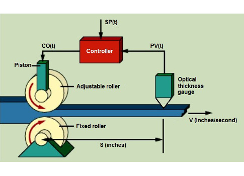
Consider, for example, the rolling mill shown in the "Simplified Deadtime Example" which produces a continuous sheet of some material at a rate of V (inches per second). A feedback controller uses a piston to modify the gap between a pair of reducing rollers that squeeze the material into the desired thickness. The deadtime in this process is caused by the separation S between the rollers and the thickness gage.

The controller in this example can compare the current thickness of the sheet (the process variable, PV) with the desired thickness (the setpoint, SP) and generate an output (CO), but it must wait at least D = S/V seconds for the thickness to change. If it expects a result any sooner, it will determine that its last control effort had no effect and will continue to apply ever-larger corrections to the rollers until the sensor begins to see the thickness changing in the desired direction. By that time, however, it will be too late. The controller will have already overcompensated for the original thickness error, perhaps to the point of causing an even larger error in the opposite direction.

How badly the controller overcompensates depends on how aggressively it is tuned and on the difference between the actual and the assumed deadtime. That is, if the controller assumes that the deadtime is much shorter than is actually the case, it will spend a much longer time increasing its output before successfully effecting a change in the process variable. If the controller is tuned to be particularly aggressive, the rate at which it increases its output during that interval will be especially high, and the resulting overcompensation will be particularly severe.

Detuning the controller

The preferred method for curing a deadtime problem is to physically modify the process to reduce deadtime. In the rolling mill example, this could be accomplished by moving the thickness gage closer to the rollers or by running the sheet at a higher velocity.

But if deadtime cannot be cured by relocating the sensor or speeding up the process, its symptoms can still be addressed by modifying the control algorithm. The simplest method is to de-tune the controller to slow its response rate. A de-tuned controller will not have time to overcompensate unless deadtime is particularly long.

The integrator in a proportional-integral-derivative (PID) controller is particularly sensitive to deadtime. By design, its function is to continue ramping up the controller’s output so long as there is an error between the setpoint and the process variable. In the presence of deadtime, the integrator works overtime. Ziegler and Nichols determined that the best way to de-tune a PID controller to handle a deadtime of D seconds is to reduce the integral tuning constant by a factor of D2. They also found that the proportional tuning constant should be reduced by a factor of D. The derivative term is unaffected by deadtime since it only comes in to play after the process variable has begun to move.

De-tuning can restore stability to a control loop that suffers from chronic overcompensation, but it would not even be necessary if the controller could first be made aware of the deadtime, and then endowed with the patience to wait it out. That is essentially what happens in the famous Smith Predictor control strategy proposed by Otto Smith in 1957.

Removing deadtime from the loop

Smith’s strategy is shown in the "Smith Predictor" block diagram. It consists of an ordinary feedback loop plus an inner loop that introduces two extra terms directly into the feedback path. The first term is an estimate of what the process variable would look like in the absence of any disturbances. It is generated by running the controller output through a process model that intentionally ignores the effects of disturbances. If the model is otherwise accurate in representing the behavior of the process, its output will be a disturbance-free version of the actual process variable.

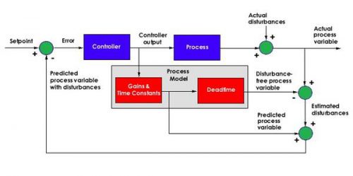
The mathematical model used to generate the disturbance-free process variable consists of two elements hooked up in series. The first element represents all of the process behavior not attributable to deadtime. The second element represents nothing but the deadtime. The deadtime-free element is generally implemented as an ordinary differential or difference equation that includes estimates of all the process gains and time constants. The second element of the model is simply a time delay. The signal that goes in to it comes out delayed, but otherwise unchanged.

The second term that Smith’s strategy introduces into the feedback path is an estimate of what the process variable would look like in the absence of both disturbances and deadtime. It is generated by running the controller output through the first element of the process model (the gains and time constants), but not through the time delay element. It thus predicts what the disturbance-free process variable will eventually look like once the deadtime has elapsed, hence the expression Smith Predictor.

Subtracting the disturbance-free process variable from the actual process variable yields an estimate of the disturbances. By adding this difference to the predicted process variable, Smith created a feedback variable that includes the disturbances, but not the deadtime.

So what?

The purpose of all these mathematical manipulations is best illustrated by the "Smith Predictor Rearranged" block diagram. It shows the Smith Predictor with the same blocks arranged to yield the same mathematical results, only computed in a different order. This arrangement makes it easier to see that the Smith Predictor effectively estimates the process variable (including both disturbances and deadtime) by adding the estimated disturbances back into the disturbance-free process variable. The result is a feedback control system with the deadtime outside of the loop.

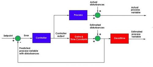
The Smith Predictor works to control the modified feedback variable (the predicted process variable with disturbances included) rather than the actual process variable. If it is successful in doing so, and if the process model does indeed match the process, then the controller will simultaneously drive the actual process variable towards the setpoint, whether the setpoint changes or a load disturbs the process. The deadtime becomes irrelevant.

Unfortunately, in the real world, those are big ifs. It is certainly easier for the controller to meet its objectives without having to deal with the deadtime, but it is not always a simple matter to generate the process models required to make this strategy work. Even the slightest mismatch between the process and the model can cause the controller to generate an output that successfully manipulates the modified feedback variable, but drives off the actual process variable into oblivion. There have been several fixes proposed to improve on the basic Smith Predictor, but deadtime remains a particularly difficult control problem.

Vance VanDoren, PhD, PE, is a contributing content specialist for Control Engineering. 

Key concepts:

• Deadtime in a process can cause a controller to overreact to a disturbance or setpoint change.
• If it isn’t practical to wait for a time interval to pass, there are techniques designed to make changes more quickly.

ONLINE

Read more on control strategy and loop tuning below.

Do you have experience and expertise with the topics mentioned in this content? You should consider contributing to our CFE Media editorial team and getting the recognition you and your company deserve. Click here to start this process.