PLC-based Bode loop analysis for industrial controls

Bode loop analysis has long been a staple in the electronics world, but due to expense and complexity of the specialized equipment involved, Bode loop analysis has not been as common in the industrial controls field. Today’s higher-performance PLCs can do Bode analysis in the PLC logic with none of the traditional expense or complexity. (Online extra: this pictorial tutorial is an online expansion of a two-page article in January 2012 Control Engineering North American print and digital edition.)

Although it may sound trivial, to maintain the stability of a negative feedback loop, the feedback must remain negative. If at any frequency the total phase shift of the loop becomes 360 degrees, the negative feedback becomes positive feedback and the loop becomes unstable. Since the subtraction in the feedback loop represents 180 degrees itself, the other loop components must contribute less than the remaining 180 degrees.

Figure 1, above, shows how the loop becomes unstable when the total loop shift is 360 degrees and the loop gain is 2.0. Courtesy: GE Intelligent Platforms

Unlike the simplified Figure 1 diagram, the gain and phase of each block of a control loop can vary with frequency and operating point. (The impact of operating point will be covered in a later section.)

Figure 2 shows the control blocks of a typical control loop with frequency-dependent components. Courtesy: GE Intelligent Platforms

Ideally, the plant we are attempting to control would have infinite bandwidth (in other words, the plant would exhibit no frequency-dependent behavior throughout the frequency range of interest). Unfortunately, this is rarely the case. At some frequency, the plant begins to exhibit non-ideal behavior, typically consisting of multiple high- and low-pass filters at various filter frequencies. For the purposes of this example, the plant will be modeled with a fixed gain of 1.0 (Gain2=1.0) and a low-pass filter effect at frequency 10 Hz (F2=10 Hz).

A single-element low-pass filter such as this plant filter will exhibit zero degrees of phase shift well below its filter frequency (F2), 45 degrees at its filter frequency, and 90 degrees well above its filter frequency. Likewise, its gain will be Gain2 at low frequency, Gain2/√2 at its filter frequency, and Gain2/frequency at high frequencies.

If the plant consists of two or more low-pass filters, each can contribute 90 degrees and their sum can reach 180 degrees and drive the control loop unstable. A common method to avoid this is to incorporate a “Dominant Pole” into the Loop Compensation block. The Dominant Pole consists of a single-element low-pass filter at a frequency which is much lower than any filter in the plant. The object is for the effects of this filter (over which we have control) to dominate the filters in the plant (over which we typically have no control).

For the purposes of this example, we will place the dominant pole at 1 Hz (F1) with a gain of 10 (Gain1). Figure 3 shows the phase and gain contribution of dominant pole and the plant, and shows how the total gain drops below 1.0 (0.0 dB) well before the total phase reaches 180 degrees (360 when the subtraction is included).

Figure 3: Gain and phase of loop components, and phase at unity gain; Courtesy: GE Intelligent Platforms

Generally, the higher the gain, the better the control loop will be able to maintain the process variable (output) to the desired the setpoint (input). But this is a bit of a balancing act. If we change the gain of the loop compensation from 10 to 20, as shown in Figure 4, the phase shift around the loop rises from 120 degrees to 137 degrees. As described further in the next section, the trade-off for this improved accuracy will come at the price of ringing on step changes. It’s the control engineer’s job to manage this balance, as well as to employ other techniques to provide the necessary accuracy while maintaining the necessary stability.

Figure 4: Gain and phase with higher loop gain; Courtesy: GE Intelligent Platforms

Bode loop analysis

Bode analysis is the process of measuring the total gain and phase shift around the loop at various frequencies and then determining margins available before the system goes unstable. These margin numbers provide a good summary of the stability of the loop.

Phase margin is defined as 360 degrees minus the phase of the loop where the magnitude of the loop reaches unity, and gain margin is the gain where the total loop phase reaches 360. A loop with phase margin greater than zero (phase shift of less than 360 degrees) will be stable, but the closer the phase margin is to zero, the more the loop will “ring” during a step change. As a rule of thumb, a phase margin of 45 degrees typically provides good stability with some ringing on step changes. A phase margin of 60 degrees usually provides very good stability with little or no ringing on step changes. Figure 3 shows the Phase margin measurement for the control system example.

Beware that in some cases the effective loop gain will decrease when a component reaches the limits of its range (saturates). For instance, notice the phase margin of the loop shown in Figure 5 will drop to near zero (at 0.1 Hz) if the gain decreases by 25 dB. If a step change drives any of the components in this loop near saturation, the loop may ring at 0.1 Hz until the ringing settles to the point where the loop components are all operating in their linear range.

For this reason, the automated phase margin measurement built into the Bode analyzer block described below defines phase margin as 360 minus the greatest phase shift encountered while the loop gain is greater than unity. Under this definition, the phase margin of the loop in Figure 5 will be roughly 5 degrees.

Figure 5: Typical Bode plot showing gain and phase margin; Courtesy: GE Intelligent Platforms

Bode analysis of nonlinear systems

Very few physical devices are perfectly linear throughout their operating range. A transfer function of a linear device would be a straight diagonal line.

Figure 6 shows the transfer function of a nonlinear device; Courtesy: GE Intelligent Platforms

Notice that the gain of the transfer function is less than 1.0 on the ends of the operating range, and up to 2.0 in the center.

Bode analysis is a purely linear measurement. If the system is nonlinear, the loop could be stable in some operating ranges but not in others. For that reason, it is important to run the loop analysis in all the operating ranges of the loop components.

The Bode analysis of a nonlinear system is performed by executing a series of Bode analyses while the dc setpoint of the system is sequentially increased as shown in Figure 7; Courtesy: GE Intelligent Platforms

While simple linear Bode analysis can be thought of as analyzing the characteristics of a vector, nonlinear Bode analysis can be thought of as analyzing the characteristics of a surface. This can be illustrated by first calculating the gain of the transfer function as a function of the input (in other words, taking the derivative of the transfer function).

Figure 7, above, shows transformation; Courtesy: GE Intelligent Platforms

The results of the transformation for the graph in Figure 7 are shown in Figure 8.

 

Figure 8: Transfer function in gain versus input format; Courtesy: GE Intelligent Platforms

Applying this gain transfer function to the plant in Figure 2 and performing a loop analysis at several dc setpoints yields the family of curves shown in Figure 9.

Figure 9: Magnitude response at several setpoint levels; Courtesy: GE Intelligent Platforms

Figures 8 and 9 are combined to form the surface graph in Figure 10, with the vertical axis being the gain, horizontal axis being frequency, and the axis into the page being the dc setpoint level. A similar graph could be generated for the phase response (but would not be very interesting since none of the blocks in this example exhibit any phase variation due to the dc setpoint).

Figure 10: Surface plot of nonlinear control system response; Courtesy: GE Intelligent Platforms

Picking out the phase and gain margins of two surfaces can be difficult, so the automated system described below includes an automatic measurement of the phase margin for each setpoint.

Logic configuration Bode loop analysis

Figure 11 shows an overall picture of where Bode analysis block fits into a typical PLC-based control system. The diagram shows the analyzer block inserted directly into the signal path. While at first this may seem counterintuitive, the logic behind this placement will be will be explained in the next few paragraphs.

Figure 11: Typical application of the Bode analyzer block; Courtesy: GE Intelligent Platforms

Figure 12: Easiest measure of gain and phase around a loop is to insert a stimulus generator and signal analyzer; Courtesy: GE Intelligent Platforms

The simplest way to measure the gain and phase around a loop would be to break the loop at some point and insert a stimulus generator and signal analyzer in the break as shown in Figure 12. Unfortunately, this configuration is not often feasible due to high loop gains, the difficulty in setting quiescent points throughout the range of the loop, nonlinearities, noise, and the danger of disabling a control loop in an operating plant.

Figure 13: Method for open-loop measurement without opening the loop; Courtesy: GE Intelligent Platforms

A technique that avoids these drawbacks is shown in Figure 13. This method allows open loop measurements to be made without actually opening the loop. This is accomplished by inserting a sine-wave signal source into the break in the loop, and then measuring the resulting signal on the upstream and downstream sides of the break. The sine-wave source has zero dc value, so as far as the loop is concerned, it’s a short circuit. The small signal from the ac source then perturbs the loop so that its response can be measured. However, the measurement is a little more involved than shown in the figure. This will be explained in detail in the next section.

Correlating signal analysis

The Bode analyzer uses RMS and correlating frequency analysis measurement techniques. Correlation is highly effective at rejecting any signal or noise that is not generated by the stimulus. Correlation involves multiplying the measured signal by the stimulus signal at every time step. The results of these multiplications are then summed and averaged.

Figure 14: Reject noise and other uncorrelated signals; Courtesy: GE Intelligent Platforms

Figure 15: The more cycles can be integrated, the better the noise rejection; Courtesy: GE Intelligent Platforms

Figures 14 and 15 shows how this technique rejects noise and other uncorrelated signals. The more cycles that can be integrated, the better the noise rejection will be. This technique is also highly effective at measuring the fundamental component in pulse width modulated and other complex modulated signals.

Simple RMS measurement includes all uncorrelated signals as well as the correlated signals. Since uncorrelated noise and signals can drive an otherwise stable loop unstable, it is wise to compare the RMS to the correlated results as a measure of the noise in the system.

PLC function block for automated Bode analysis

With today’s high-performance PLCs, the Bode analysis calculations can actually be performed directly on the PLC in the PLC logic. This capability eliminates the need for expensive external equipment and complicated wiring, and makes Bode analysis much more accessible to control systems engineers.

Figure 16, above: How to insert a Bode analyzer block into a control loop; Courtesy: GE Intelligent Platforms

Figure 17: How an inserted Bode analyzer block looks in ladder logic; Courtesy: GE Intelligent Platforms

Figure 16 shows diagrammatically how a Bode analyzer block would be inserted into a control loop, and Figure 17 shows how this would look in Ladder Logic. The block provides both the stimulus (SineIn and SineOut) and the measurement (BodeIn and BodeOut), as well as the dc voltage to bias the system nonlinear analysis as described earlier (SetPointOut).

In Figure 17 the TestParams input provides a connection to a UDT (user defined type) that contains the test parameters (dc steps, frequency steps, settling time, etc.) and tables in which to place the resulting measurements.

Figure 18 shows a UDT that stores both the specifications for the Bode loop analysis as well as space for the analyzer to place the results. The results can be plotted directly with PLC-based HMI software, or can be read from the PLC via Ethernet and plotted in Matlab, Excel, or such.

To be able to see the full structure, the UDT has been reduced to only three setpoints and three frequency steps. A typical analysis would involve many more setpoints and frequency steps.

Figure 18, above: Analysis specifications and analysis results are stored in a UDT variable. Courtesy: GE Intelligent Platforms

Figure 19: The same function block can measure closed-loop response. Courtesy: GE Intelligent Platforms

The same function block can also be used to measure the closed-loop response as shown in Figure 19. In this case, the stimulus is added to the dc bias before it applied to the control input. The measurement is made from the control input to the plant output. See Figure 25 for sample results of a closed loop measurement.

Figure 20 opens the function block for open-loop response. Courtesy: GE Intelligent Platforms

The same function block can also be used to measure the open loop response of control loops, which can be opened as shown in Figure 20. In this case, the stimulus is added to the dc bias before it is applied to the plant. The measurement is made from the control output to the plant input. Figure 21 shows a variation of the block that provides multiple measurement points, loop degradation alarming, and dynamic loop parameter control. Multiple inputs allow the gain and phase to be measured between any two points in the loop, which is very useful for identifying the source of unexpected loop behavior while using only a single analysis run. For processes that can tolerate minor perturbation or have downtime between batches, the block can be used dynamically measure the performance of the loop and either provide an alarm to the operator or potentially apply optimizing adjustments to the loop components themselves.

Figure 21: Multi-input block with auto loop analysis, alarm, and adjust; Courtesy: GE Intelligent Platforms

Internals of the Bode analysis function block

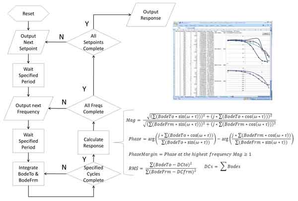
The flowchart on the left of Figure 22 shows the overall operating sequence of the Bode analyzer block, and the equations on the right side show the analysis that is performed at each frequency step. (See Figure 18 for how the test parameters are specified.)

Figure 22, on the left side of the graphic, shows a flow chart with operating sequence of the Bode analyzer block. On the right are equations with analysis performed at each frequency step; Courtesy: GE Intelligent Platforms

The following code excerpt shows the operation executed on each PLC scan in the “Integrate BodeTo & BodeFm block”:

Sine = sin(PhaseAccumulator);

Cosine = cos(PhaseAccumulator);

rTo += (MeasureTo – QuiescentTo) * Sine;

jTo += (MeasureTo – QuiescentTo) * Cosine;

rFrom += (MeasureFrom – QuiescentFrom) * Sine;

jFrom += (MeasureFrom – QuiescentFrom) * Cosine;

AvgTo += MeasureTo;

AvgFrom += MeasureFrom;

RMSTo += (MeasureTo – QuiescentTo)*(MeasureTo – QuiescentTo);

RMSFrom += (MeasureFrom – QuiescentFrom)*(MeasureFrom – QuiescentFrom);

PhaseAccumulator += PhaseStep;

SineOut = SineIn + TestParameters->Amplitude * sin(PhaseAccumulator);

The first two lines create the sine and cosine of the stimulus using phase accumulation. The next four lines accumulate the product of the stimulus and measurements, and the following four lines accumulate the Average and RMS measurements. The last two lines increment the phase accumulator and output the next point in the stimulus waveform. Phase accumulation is used to avoid discontinuities in the waveform when stepping from one frequency to the next.

Note that the quiescent points are subtracted from the measurements before they are integrated. The quiescent points would typically be averaged out of the calculation during the integration process, but in the meantime it can cause numerical precision problems.

The next excerpt shows the operation performed in the “Calculate Responses” block of Figure 22, which is performed at each frequency step:

Magnitude = 20.0*log10((sqrt(rTo*rTo+jTo*jTo)/(sqrt(rFrom*rFrom+jFrom*jFrom))));

Phase = UnwrapPhase((180.0/pi)*arg(jTo,rTo),(180.0/pi)*arg(jFrom,rFrom));

RMS = 20.0*log10(sqrt(RMSTo/RMSFrom)); //Calculate the Phase Margin (only when below 30% of Nyquist)

if (Frequency <= 0.3/TestParameters->ConstantSweepPer)

if ((abs(QuiescentTo – AvgTo/TotalSamples)/QuiescentTo > .0001)

FreqStep++; //go to the next frequency step PhaseStep = 2.0 * pi * FreqValues[FreqStep] * ConstantSweepPer / TotalSamples;

The first three lines calculate the magnitude, phase, and RMS values of the differential between BodeTo and BodeFrom. UnwrapPhase keeps track of phase as it wraps around 360 degrees. The next several lines calculate the Phase Margin as described earlier in the article.

The next lines verify the value of “QuiescentTo” and “QuiescentFrom” subtracted from the accumulations above. The quiescent values are determined by taking samples of the BodeTo and BodeFm after the SetPoint settling time and before the first stimulus point is generated. These quiescent values are compared to the average values calculated during the sweep. If the system is noisy or slightly unstable, the values might not match and the sweep values might not be valid.

The last lines calculate the new PhaseStep value that will be used to generate the next stimulus signal.

Bode analysis test results

The Bode analyzer was tested in several ways. First, IIR models created for the loop compensation and the plant blocks and the system were simulated on the PLC with the Bode analyzer inserted as shown in Figure 23.

Figure 23 Bode analyzer testing; Courtesy: GE Intelligent Platforms

The model for the Control (subtraction and loop compensation) is shown in the following code excerpt:

const T_REAL64 a = tan(pi*Fpole*Tscan) / (tan(pi*Fpole*Tscan)+1.0);

const T_REAL64 b = (tan(pi*Fpole*Tscan)-1.0) / (tan(pi*Fpole*Tscan)+1.0);

static T_REAL64 xv[2], yv[2];

xv[0] = xv[1]; xv[1] = SetPoint-Feedback;

yv[0] = yv[1];

yv[1] = (xv[0]+xv[1])*a – yv[0]*b;

return(yv[1] * Gain);

The plant model is similar, except it also includes a function that can be switched on to add a small amount of nonlinearity to the model as described in the following code excerpt:

if (x < Vlow) x = x*Glow; //Constant gain1

else if (x < Vhigh)

else x = x*Ghigh+Ghighoff; //constant gain2

The loop compensation has a gain of 10 with a pole at 1Hz, and the Plant has a gain of 1.0 with a pole at 10Hz. The sampling rate is 100Hz.

The first check was to verify the results with that expected for the system with the poles and zeros as modeled. Then, the RMS results were verified against the correlated results. Since the system at that point didn’t contain any noise or nonlinearities, the RMS and correlating results should match identically.

Then, linear S-parameter models were added to the system, and the results were compared to that expected with linear models. The linear models did include group delay effects, but did not attempt to include any aliasing effects. So, the linear and IIR simulations will begin to diverge at roughly 40% of Nyquist. The S-parameter model uses complex math, as shown in this code excerpt:

_Complex double Xfer = – ( (Gain/(1.0+1.0if*f/Fpole)) *

Figure 24, below, shows the results of the correlating, RMS, and S-parameter simulations as described above.

 

Figure 24: Correlating, RMS, and S-parameter simulations; Courtesy: GE Intelligent Platforms

The difference between the IIR (Mag, RMS, and Phase) diverges from the linear model (S-Param) at roughly 40% of the Nyquest frequency as described above. Generally speaking, it’s not advisable to run a control loop anywhere near its Nyquist frequency, so this isn’t normally an issue. The spike in the phase results at the Nyquist frequency is a result of the phase unwrapping algorithm becoming confused with the rapid change of phase at that point.

 

Figure 25: Simulation results using nonlinear plant model; Courtesy: GE Intelligent Platforms

Figure 25 shows the results of the simulation using the nonlinear plant model. This analysis graphically shows the importance of the performing the Bode analysis throughout the operating range of the system. Notice that the phase margin varies from 63 to 44 degrees. At 44 degrees the closed loop results show peaking, which will also correspond to ringing in the time domain as explained in the first chapter.

Real-life Bode analysis results

The Bode analyzer function block described above was used to analyze and improve the control loop used on a gas turbine engine. The turbine manufacturer evaluated and approved the Bode analysis function block for use with certifying the turbine control systems. Figure 26 shows a snapshot of one of the analyses performed while the control loop was being adjusted and optimized. In this case, five setpoint steps were used.

Figure 26: Gas turbine control analysis results; Courtesy: GE Intelligent Platforms

– Gary L. Pratt, PE, is applications manager for GE Intelligent Platforms.

www.ge-ip.com 

https://www.controleng.com/tutorials 

Do you have experience and expertise with the topics mentioned in this content? You should consider contributing to our CFE Media editorial team and getting the recognition you and your company deserve. Click here to start this process.