How to automate: Using a valve characterizer example, learn how proportional-integral-derivative (PID) control can reach outside of usual linear processes to effectively handle real-world, non-linear applications.
Learning Objectives
- Understand that some non-linear systems can be controlled more reliably by making them linear for PID controllers.
- Valve characterizer improves PID control effectiveness.
- Tables and graphics help explain a PID tutorial.
PID for valve control insights
- Some non-linear PID systems can become more reliable by making them linear.
- Valve characterizer example shows how to improve PID control effectiveness.
- Tables and graphics help explain a loop tuning tutorial, increasing reliability for PID applications that may be non-linear.
- This method of tuning valve characterizer is applicable to non-integrating processes which are inherently stable when the controller is in manual mode.
One of the most common difficulties when working with proportional-integral-derivative (PID) control is PID control (CO) is designed to work with a linear process. However, in real world applications, many process variable (PV) responses show non-linear behavior. The more non-linear the system response is, the more difficulty a PID algorithm will have in controlling the system.
For help applying PID control to a non-linear process, follow these suggestions for processes that are non-integrating and are inherently stable when their controller is put into manual mode
Resolve process non-linearity
One of the most common ways to try to resolve this process non-linearity is to build a valve characterizer to adjust for the process non-linearities. This method linearizes the process to the PID controller so the PID sees a linear process response to the PV even though the actual process is non-linear. The figure shows a valve characterizer flowchart.

Build a valve characterizer
To build a valve characterizer correctly, look at the percent PV to the percent CO and think of the PV in percent instead of engineering units. That way, when doing the reverse conversion, the calculated valve demand will be in percent.
Initial full-range response
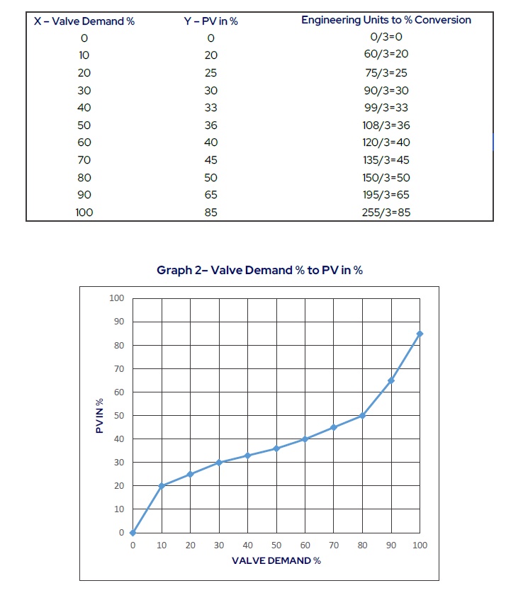
As an example, begin with a process that has been trended with CO values mapped for every 10% change in CO and shows the corresponding PV in engineering units (EU in table). Since there is no characterizer configured yet, the CO is equal to the valve demand. The profile developed for this loop is as follows in Table/Graph 1.

Convert to PV in percent
Next, convert the PV in engineering units to PV in percent. In this example, the PV maximum value is 300 and the PV minimum value is 0, so the scale to convert from engineering units (EU) to percent (%) is (100-0) / (300-0) = 1/3. So, 100 EU = 100/3 = 33.3%, 150 EU = 150/3 = 50%, etc.
Now convert this simple table of valve demand to PV in percent that looks something like Table/Graph 2.
Linearize the PID response by creating a valve characterizer curve
Next, set the CO = PV to linearize PID controller response. Doing so provides a graph of valve demand percent to PID CO percent. Then, create a reverse or inverse profile linearization of Graph 2 by flipping the X and Y axis, as shown in Table/Graph 3.

When comparing Graph 2 and Graph 3, note they are the inverse of each other. Graph 4 combines them to see the inverse trends more clearly.

In graph 4, the gray line is linear. By using the orange profile for the CO% to Valve Demand %, it will create a PV response that linearizes the PV signal to the CO, so for every desired CO out, the PV shows the same percentage out.
Consider the curve that maps CO% to valve demand %. There’s a lot of data in the range of 20 to 50% of the valve demand, but the linearization is sparser when outside of this range.
Now add new points to the curve using the method of linear interpolation. For example, at 10% CO, the linearly interpolated valve demand is 5%. Insert a new point to the curve that 10% CO renders 5% valve demand. The Table before Graph 5 has more defining points at CO equal to 10, 60, 70 and 80%.
It is important to note the original set of points defining the valve characterizer curve are obtained by testing the process, whereas newly inserted points are obtained by method of linear interpolation and play the role of placeholder points for fine-tuning the curve after its implementation.
The valve characterizer generated from Table 4 can be implemented with a linearization block where PID CO% is the X value, and valve demand percentage is the Y value.

Update the valve characterizer curve
Once in operation, it’s possible the curve does not linearize PID response as accurately as needed due to process shifts in time or due to operating at regions where the curve is defined by means of linear interpolation instead of process testing. Next, see a method to update the in-place valve characterizer curve to improve linearization of the PID response.
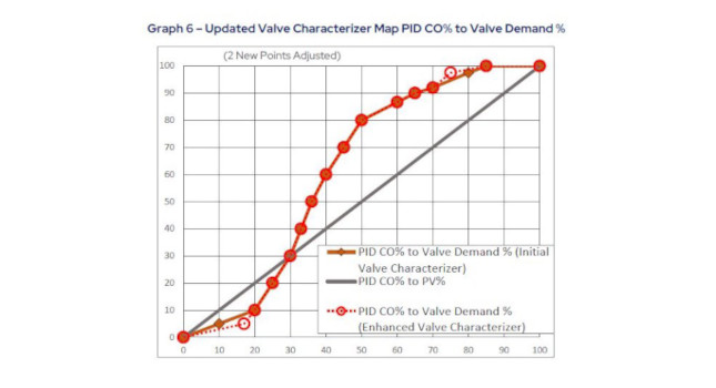
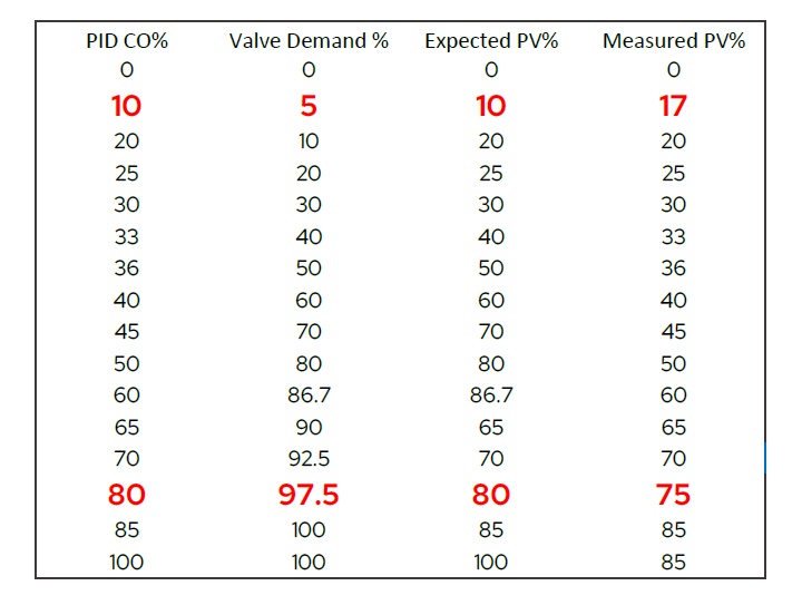
Consider the valve characterizer of Graph 5 where for 10% PID CO, the valve demand is 5%. A PID CO of 10% would be expected to produce a PV response of 10%. However, this point in the curve was not based on process testing, so the actual measured PV could differ from 10%. To test this, put the CO demand at 10% and assume the actual PV value at 5% and valve demand is 17%. Update the table to include this latest information.
The top of the linearization curve has the same issue. When the PID CO goes above 70%, the response of the curve is not as good as expected. Setting the PID CO to 80% generates a valve demand of 97.5%, which would be expected to result in a PV of 80%, however, the actual PV response instead is 75%.
A summary of updated findings from Graph 5 is shown in Table 5a.
Since this exercise is attempting to map CO%=PV% (that is, linear), the PID CO% needs to change to match the actual PV% measured. Graph 6 is updated with this added information.

Matt Petras is senior control application engineer and author, with contributions from Alireza Haji-Valizadeh Ph.D., technology development director, both with ControlSoft. Edited by Mark T. Hoske, content manager, Control Engineering, CFE Media and Technology, [email protected].
KEYWORDS: Proportional-integral-derivative, PID tutorial
CONSIDER THIS
Loop tuning: What non-linear PID applications could be more reliable with this method?
ONLINE
www.controleng.com/control-systems/pid-apc