Instead of wasting the potential energy associated with the BackEMF voltage of a vehicle's electric motor via heat loss, it can be used to recharge the battery and therefore recover energy for higher system efficiency. Certain manufacturing processes can be made more efficient in similar ways. See diagrams, graphics, and equations.
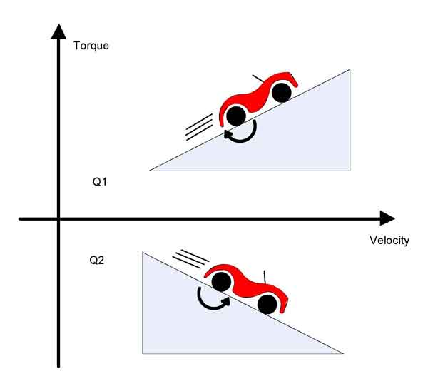
In the motion control industry, the term “regeneration” or “regenerative braking” refers to using the power associated with the BackEMF (back electromotive force) voltage of an electric motor to charge a battery. This is the opposite of the normal operational mode where the battery is used to provide power to an electric motor. However, since an electric motor can act as a generator, a system can be designed where the power flow (in or out) of the motor and battery can change in real time. So, instead of throwing away the BackEMF power into heat loss, it can be used to recharge the battery, thereby recovering energy, adding to overall system efficiency. See Figure 1 below.
Gravity testing
Many motor/battery systems have the potential for regeneration including those used for manufacturing. In battery-powered vehicles that use a permanent magnet motor as the drive, the system is simple with an intrinsic steady-state regeneration condition (until the bottom of the hill is reached). The drive system will operate in all “four quadrants,” meaning the drive must be able to control both the acceleration and deceleration of the vehicle in both forward and reverse. At steady state there exists the possibility to use the motor’s BackEMF voltage to recharge the battery in two of the four quadrants. Under the right conditions this can make a significant contribution to the system’s power efficiency in the context of extending the time between battery charges.
Figure 1 shows the vehicle operating in two of the four quadrants, one being positive velocity/ positive torque, the other being positive velocity/ negative torque. The other two quadrants can easily be realized by reversing the sign of velocity. The direction of rotation of the motor will determine the sign of the motor’s BackEMF voltage, and the magnitude of the velocity will determine the magnitude of the motor’s BackEMF voltage.
In Figure 1, the motor’s BackEMF voltage is always positive and increases in magnitude with speed. It is assumed that the vehicle moving uphill will always need a “positive” torque as indicated by the direction of the arrow. The vehicle moving downhill requires a “negative” torque from the motor to brake the car and prevent a runaway condition.
Motor model
Figure 2 demonstrates the standard single-phase motor model (resistive, inductive, and BackEMF components) whereby positive current flow corresponds to motor torque in the positive direction. The polarity relationship between the battery voltage and motor’s BackEMF voltage stems from that current flow convention. (The polarity of the motor’s BackEMF voltage is rotation direction dependent and will oppose the direction of current flow that generates torque in the same direction.) See Figure 2 below.
Control of the vehicle under the given conditions requires proportional control of the current in the motor. This is achieved by using a voltage regulation scheme that can apply a portion of the battery voltage to the motor with either positive or negative polarity. This proportional voltage is referred to as an “effective voltage” (Veff). This concept is the foundation for common servo motor drives (linear and PWM switching) where proportional control is required. The effective voltage, along with the motor components, is used in the standard electrical motor equation, which can be derived from Figure 2 after substituting effective voltage for the battery voltage.
Where does regeneration live?
All points in quadrant 2 (see Figure 1) correspond to a condition referred to as “dynamic braking.” The motor current is producing torque in the direction that opposes motion (hence the “brakes” are being applied). The emotive force behind that current could be the battery or the BackEMF and, in almost all cases, is a result of both.
For the steady-state condition, quadrant 2 can be further divided based on the sign of the effective voltage, Veff, which is determined by the controller to yield a specific motor current. The region in quadrant #2, where the effective voltage is positive (opposing the BackEMF), is where “regenerative” braking takes place (not just “dynamic” braking). Refer to Figure 3 for an illustration of this. In the case of transient operation, regeneration can occur anywhere within the operating range. See Figure 3 below.
This is also the one and only steady-state region where current is flowing into the positive terminal of the battery. Assuming the duration of time spent in this region is significant, this condition equates to electrical power flow into the battery and hence the battery is “recharging.” In the given system, the path of energy exchange begins with gravitational energy (elevation change) conversion into kinetic energy, which includes the rotational energy of the vehicle’s wheels. The wheel rotation translates into a motor rotation and subsequent BackEMF voltage, which, under specific conditions, results in current flow into the positive battery terminal.
Up until now the left-hand side of Figure 3 has not been discussed. In this half, the velocity is negative and therefore the BackEMF voltage is also negative. The polarity relationship between BackEMF voltage and effective voltage is preserved. In the case of negative BackEMF voltage, the effective voltage must also be negative and the current must be positive for regeneration to occur at a steady state.
Figure 3 was derived for the given system but is valid for simple inertial systems driven by a motor operating at steady state. In other systems, external forces could alter the location of the operational envelope defined there.
H-bridge analysis
An H-bridge is the most common scheme used to implement a four-quadrant PWM controller on a brushed dc servo motor. The PWM duty cycle controls the proportion of the supply voltage (battery) that the motor is exposed to, which has been previously referred to as the effective voltage.
A steady-state analysis will be performed at a point in the positive velocity regeneration region. The motor winding current at steady state can be expressed in terms of effective voltage, BackEMF voltage and winding resistance.
The steady-state selection point results in the following requirements:
- Veff > 0
- Vemf > 0
- Vemf > Veff
- Vbatt > Vemf + RI
A motor controller will control the effective voltage to the motor by controlling the four MOSFETs (metal-oxide-semiconductor field-effect transistors) of the H Bridge shown in Figure 4, below.
Various switching schemes exist for controlling the four MOSFETs, one of which will be used here. We now join the PWM cycle with the system at a steady state with an average negative current (opposite the direction shown in Figure 4), positive BackEMF voltage, and positive effective voltage. Looking inside the PWM period there are four MOSFET drive states occurring over one PWM cycle, in this order:
1. High sides off / low sides on
The current is recirculating in the lower MOSFETs. The BackEMF voltage causes the current to become more negative as the inductive energy stored in the motor windings is resistively dissipated. There is no flow to/from the battery and therefore no regeneration. The current will decrease at a rate of:
2. Opposing MOSFETs on
Which pair of the MOSFETs depends on the sign of the effective voltage the controller wishes to apply. In this case (+Veff), the upper left and lower right MOSFETs will be conducting. Since the remaining MOSFETs are not conducting, there is only one path for this negative current, which is back into the battery. The current will drift toward zero while energy is being dissipated in the resistive components as well as flowing into the battery. This is a state of regeneration and the battery is being charged. The current will decay at a rate of:
Note: Vbatt is the true battery voltage, not to be confused with effective voltage (Veff)
To simplify this proof, the battery is treated as an ideal power source with infinite current sink/source properties. The effects of battery efficiency will be discussed later.
3. High sides on / low sides off
Identical to the first state with the exception that the current is recirculating in the upper MOSFETs.
4. Opposing MOSFETs on
Identical to state 2, another case where regeneration is taking place. At the end of this state the PWM cycle has completed. Since a steady-state system has been defined, the instantaneous current will be equal to the instantaneous current at the beginning of state 1.
We have seen that in states 2 and 4, current is flowing into the battery. There are no conditions where current is flowing out of the battery in this analysis. The instantaneous power delivered to the battery is the battery voltage times the current. However, if the controller was applying an effective voltage that was 25% of the battery voltage, the combined times of states 2 plus 4 would equal 25% of the total PWM period. So, the average power delivered to the battery will be the battery voltage times the current times the duty cycle percentage.
Mechanical model
The analysis will be continued by creating a mechanical model of the electric vehicle. The model will be simplified by adhering to rigid body analysis only. This implies that elastic deformation of components like axles and drive shafts will be ignored and assumed to be zero. Additionally, there will be no frictional components included in the model, which implies the wheel and motor bearings are ideal and the gearing mechanism has no efficiency loss. This also implies that there is no wind drag on the model. This model can be used to gain insight into the nature of the energy recovery; however, if a real-world numerical estimate of the amount of energy recovered is required, the frictional and efficiency components need to be accounted for properly in the modeling process.
The model of the electric vehicle will be defined by a set of mechanical and electrical parameters. Figure 5 below defines two of these: The mass of the vehicle and the slope of the hill.
To model the motion of the vehicle and the resulting energy recovery, the mechanical drivetrain of the vehicle must be analyzed. This includes the motor and a gear assembly attached to one wheel. The other three wheels are free to spin. Figure 6 below depicts the forces and torques acting on the vehicle’s drivetrain.
All translational motion of the vehicle occurs along the x-axis, which is always parallel to the road surface. The motor and motor gear rotate together as one rigid body. The “Ti+” arrow indicates the direction of torque produced by positive current. In accordance with the rotation direction defined here, this will be torque in the negative direction. F’m is the force of the wheel gear acting on the motor gear. Summing the torques about the center of the motor gear (m) results in:
Substituting Kti for Ti+ and solving for Fʹm results in:
The wheel gear and wheel are also treated as one rigid body where the rotation of the wheel gear is equal to the rotation of the wheel. The axle bearing (see Figure 6) acts on this rigid body and ultimately transfers all gravitation and translational inertial forces. Summing the forces acting on this rigid body along the x-axis results in:
Summing the torques about the center of the wheel (c) results in:
Solving for Fw:
A few system observations will allow for some useful substitutions.
- Fm = -F’m
Making substitutions in the force equation and letting Fm = -F’m:
The rotational velocity terms will now be replaced with linear velocity terms:
And then solve for:
Expansion of motor model
To facilitate use of the electrical equation in a system analysis, the BackEMF voltage will be expressed as a function of the vehicle velocity:
Substituting back into the electrical equation for the motor and solving for di/dt:
Electromechanical model
At this point, two first-order ODEs have been created, one derived from mechanical properties and the other derived from electrical properties. These can be combined to create a system of first-order nonhomogenous ODEs:
Where
This becomes the foundation for a mathematical model of the vehicle whose solution will provide an expression for the current and velocity as a function of time. The contents of matrix A and B are constants, and therefore a solution for the ODEs exists. Since the goal is to gain insight into quantifying the energy recovered, appropriate numerical values will be established for the various model parameters.
The scaling of the numerical parameters is based on a golf cart as opposed to a typical passenger vehicle. At this point Matlab from MathWorks will be used to solve the ODEs and provide numerical data that can be used to calculate power flow under specific conditions.
Table: Parameters, units, descriptions, values for electric vehicle regeneration model
Regeneration can exist as a steady-state condition. To set up the model to run under those conditions, the initial state of the vehicle is sitting on the downward slope of a hill with the parking brake engaged. The motor drive stage is disabled such that all MOSFETs are open (not conducting). This means there is no potential for current flow in the motor since there is no path for that current to flow along. The parking brake is now disengaged (t0=0), and the vehicle begins to accelerate down the hill. The motor also begins to rotate and generate BackEMF voltage; however, this does not produce any current since the MOSFETs are still open. There is no braking of any kind occurring in this state.
After 8 seconds (t1=8) the vehicle has accelerated up to about 14 mph (see Figure 7), at which point the drive stage is enabled and running with a constant duty cycle of 25%. The BackEMF voltage of the motor will now produce current since a path exists for the current to flow in. Also note that the BackEMF voltage is larger than the effective voltage, which means the current will grow negative. It reaches a value of –8 Amps almost immediately (within 8 ms) (t1+). However, this current will cause the motor to produce a braking torque that slows down the vehicle, thus reducing the BackEMF voltage. The force of gravity will keep the absolute BackEMF voltage above the effective voltage (which has opposite polarity). This will permit a steady-state condition to exist where velocity is positive, current is negative, and the effective voltage is positive (tss). Figure 7 follows.
Figure 8 shows the various states that have transpired while running this model, beginning with t0 and ending with tss. Regeneration begins as soon as the drive stage (MOSFETs) is enabled, which allows the BackEMF voltage to produce current. After about 10 seconds the speed and current are almost at steady state. The model is now in a steady-state region of regenerative braking. Figure 8 is below.
At the end of the section pertaining to the H-bridge analysis, it was concluded that the average power flow into the battery can be defined by the battery voltage times the current times the duty cycle percentage.
The steady-state current is about -4 amps and subsequently the power flow is about 48 W. However, the typical efficiency of a lead acid battery is 75%-85%. This means that only a percentage of the energy flowing into the battery will be stored as electrical energy that can be later used. The remainder of the power is lost due to thermal heating. In this case, the rate of energy being stored that can later be used is about 35-40 W. Further limitations arise as a result of battery properties, one of which being that the recharge efficiency will reach zero when fully charged.
– Tom Keller is senior applications engineer at Performance Motion Devices (PMD). Edited by Mark T. Hoske, CFE Media, Control Engineering, www.controleng.com.
Consider machine number and type, controller requirements, motor power range to choose motion controls
www.controleng.com/new-products/motors-and-drives.html