PID spotlight, part 17: Heuristic tuning of integrating processes

You are asked to tune an integrating process that is swinging nearly continuously. You’ve done all the checks to prove that it really is a tuning problem. Open loop testing is out of the question; how do you fix it? Using heuristics can help.

Heuristic PID controller tuning insights

• The controller performance goals determine how controller gain and integral are set.
• Use pattern recognition and simple rules to adjust controller tuning.
• Combine heuristics with open- and closed-loop tuning methods to speed loop tuning when possible.

---

---

Heuristic (guided trial and error) tuning of integrating processes is complicated. Not because it is difficult, but because we are tuning for a primary purpose and also have to work within secondary constraints. This means that there are not necessarily hard guidelines for what good looks like, and that two identical processes in different services may require very different tuning based on their role in the overall process.

Figure 1 is a tuning map for an integrating process with a process gain (K_p) of 0.2%/minute, three lags (T₁, T₂, T₃) of 30 seconds each, and no deadtime (D_t). This will help explain the problem we can have when tuning the most common integrating process, a level.

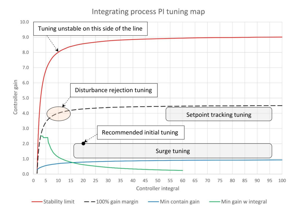
For this process Figure 1 shows us the window within which we can set the controller gain and integral for this integrating process. 

• To the left and above the black line titled “stability limit” this process is unstable. 
• The blue line titled “min contain gain” is the minimum combination of controller gain and integral that will contain a 50% change in input (or output) flow when the vessel is 50% full. This is an arbitrary convention; if you have specific process knowledge you can set your own minimum. 
• The green line titled “min gain w/ integral” is the minimum controller gain that will suppress integral driven oscillations. In PID spotlight, part 11, we learned that controller gain is required to prevent uncontrolled process swings driven by controller integral action; the faster the integral the larger the controller gain required to prevent instability. In this particular process once the integral gets below 6.0 minutes/repeat oscillations begin regardless of the controller gain setting. At this point oscillations are going to occur and get worse as integral is made faster.

The window above the blue and green lines and below and to the right of the black line is the limit of possible tuning for this controller.

Finally, the black dashed line titled “100% gain margin” is one-half the maximum stable controller gain (the black line). Above this line there will be controller gain driven oscillations, therefore normally controller gains should not much exceed this line.

For levels there are three possible performance goals. In order of frequency these are surge control, disturbance rejection and setpoint tracking tuning. We can see that each exists in its own area of the tuning window, and that the window of acceptable tuning for surge control and setpoint tracking tuning can be very wide. Tuning for each performance goal can be summarized as:

• Surge control: Minimum controller gain and slowest integral consistent with keeping the process variable within acceptable limits.
• Disturbance rejection: Maximum controller gain and fastest integral with minimum oscillation.
• Setpoint tracking: Maximum controller gain without oscillation and slowest integral with acceptable recovery from disturbances.

I will add a final caveat: If you are trying to balance multiple goals the best tuning constants may be somewhere between all three zones. 

Heuristic tuning: Too much or little, too fast or slow?

To recap PID spotlight, part 9, heuristic tuning is nothing more than pattern recognition to answer these questions:

• Is there too much controller gain or too little?
• Is the integral too fast or too slow?
• Is there too much derivative?

As discussed in PID spotlight, part 12, the visual cues used to answer these questions are:

• If a controller has too much controller gain, integral or derivative it swings. If it has too much controller gain the process variable (PV) and controller output (OP) peaks line up (or are very close). If the integral is too fast the OP peaks trail the PV peaks. 
  • If it has too much derivative the OP peaks lead the PV peaks, and the amplitude of the OP swings are usually larger than the PV swings.
• Too little controller gain will look like the integral is set too fast; the process will oscillate and the OP peak will trail the PV peak. Slowing down integral will not fix the tuning problem. It will likely make control worse. As a general rule if the controller gain (K) is less than 1.0 raise it to at least 1.0.
• Integral set too slow will not show up in a setpoint step test. Integrating processes will follow setpoint (SP) changes very well on gain only control. To check integral action, use an induced disturbance test.

Heuristic tuning methodology: Two types

There are two heuristic tuning methodologies depending on the purpose of the controller. If the purpose of the controller is setpoint response we will use the same methodology that was used for self-limiting processes:

1. Verify the process is stable and the process variable is on setpoint.
2. Change the controller setpoint (the controller is in auto).
3. Observe the process response; what pattern does it match?
4. Execute the rules for the identified pattern.
5. Repeat as necessary.

However, if we are tuning for surge control or disturbance reduction we need to induce a disturbance into the process. The methodology to do this is:

1. Verify the process is stable and the process variable is on setpoint.
2. Place the controller in manual.
3. Change the controller output.
4. Immediately place the controller back in auto.
5. Observe the process response; what pattern does it match?
6. Execute the rules for the identified pattern.
7. Repeat as necessary.

This methodology is required because of the very different way integrating processes respond to setpoint changes and disturbances. It is also assumed that the process will respond about the same way to changes in the input and output flows.

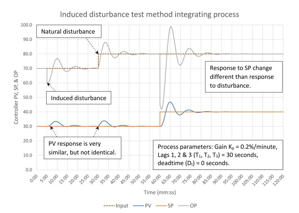
Figure 2 shows the response of an integrating process to an induced disturbance at the five-minute mark, a natural disturbance at the 30-minute mark, and a setpoint change (SP) at the 60-minute mark. The process variable (PV) response to the induced and natural response is similar but not identical. This is because the process responds immediately to an input flow change, but the response to the output flow is delayed by the three 30-second lags.

Regardless, the two responses appear to be similar enough that we should be able to draw proper conclusions from the response to an induced disturbance. The response to the setpoint change is considerably different, highlighting the need to induce a disturbance when the controller purpose is specifically intended to manage disturbances.

Three rules for too much controller gain

It is very unusual to run into a level controller with too much controller gain. Typical levels have very large fill time/deadtime ratios. If you should happen to run into a case where the PV and OP peaks line up you should check for excessive deadtime. The rules are:

• Cut the controller gain by 30% (anywhere between 25-50% will do).
  • Repeat until swinging is reduced to an acceptable level.
• If the tuning logs show the controller gain was recently raised split the difference.
• If the swing is quarter amplitude dampening or more (each peak is 25% the size of or larger than the previous peak) use closed-loop tuning rules to estimate new tuning constants.

If you end up with a controller gain below 1.0 you should take a closer look at the process. Does the process make sense? The controller may no longer be capable of keeping the process within limits.

Two rules for integral set too fast

This is the most common problem with level controllers. Inexperienced controller tuners (a much-younger me) may not understand that integrating processes are different and use self-limiting process tuning methods inappropriately. This may result in tuning that is short on controller gain and with the integral set too fast. When you run across a process where the OP peaks trail the PV peaks the rules are:

• Increase the integral by 50% (anywhere between 25% and 75% will do).
  • Repeat until swinging is reduced to an acceptable level.
• If the tuning logs show the integral was recently sped up split the difference.

Depending on the controller purpose you may want to consider raising controller gain at the same time.

Two rules for too little controller gain

This can occur through a misguided attempt at surge control tuning or an attempt to stop an integral induced swing by cutting controller gain (the standard fix for a swinging controller most young control professionals are taught). Should you run across a process with a very slow oscillation and a controller gain less than 1.0 the rules are:

• Set the controller gain using the open loop testing rules for controller gain. Be forewarned that this could go unstable if the process has a low fill time/deadtime ratio. If this is a disturbance rejection controller (unlikely if the controller gain is less than 1.0) continue to increase until a slight swing occurs, and then reduce the gain.
• If the tuning logs show controller gain was recently lowered split the difference.

Two rules for integral set too slow

If the purpose of the controller is setpoint following or surge control integral should be set to restore the PV to SP within some reasonable amount of time. There are no hard and fast rules here, although generally the integral constant should be somewhere between 10 and 50 minutes/repeat.

If, however, disturbance rejection tuning is required:

• Decrease the integral by 25% to 50%.
  • Repeat until a little swinging is detected, then increase if necessary.
• If the tuning logs show the integral was recently slowed down split the difference.

Three rules for too much derivative

Level controllers should not require derivative, therefore derivative should be set to zero. However other integrating processes may benefit from derivative if the process appears to have multiple lags. The general process is:

• Set derivative to zero.
• Verify and fix, if necessary, the controller gain and integral.
• Increase derivative stepwise until desired performance is achieved or swinging starts to occur.

Unlike self-limiting processes setting derivative to one-fourth of the integral may not work. Start with a smaller value.

Example 1: Disturbance rejection

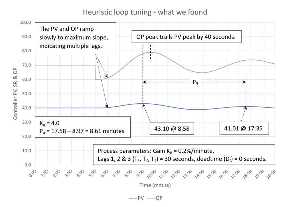
Figure 3 is a test of a process that should be tuned for disturbance rejection. The tuning is aggressive, causing the process to swing five times before settling after a disturbance. Our first assessment is while the controller output (OP) peak trails the process variable (PV) peak this looks more like a controller tuned with too much controller gain (our best guess is both are too aggressive but controller gain is the bigger problem). The amplitude damping is 32% (1.01/3.10 – peak 2 deviation divided by peak 1 deviation from SP), which is greater than quarter amplitude dampening and means we can use closed-loop tuning methods to estimate new tuning constants.

Since we do not have a continuous oscillation, we know that the current controller gain is less than the ultimate controller gain, and the current oscillation period is longer than the natural period. We can borrow from a closed-loop quarter amplitude damping tuning method a couple of equations to estimate the ultimate controller gain (K_u) and natural period (P_n).

K_u = 1.5 * K_q

P_n = 0.7 * P_q

Where:

K_q is the quarter amplitude damping controller gain

P_q is the quarter amplitude damping period

G. K. McMillan, Tuning and Control Loop Performance, eq. 1.17g, 1.17h, p.34

We’re cheating a little bit here, and if the amplitude damping was 50% or greater we would use the controller gain and period directly. Our goal is to be quick with reasonable accuracy. In this case we calculate the approximate ultimate controller gain and natural period to be:

K_u = 1.5 * 4.0 = 6.0

P_n = 0.7 * 8.61 = 6.03 minutes

We can use the second series of equations of the closed-loop simplified integrating process PI tuning calculations from PID spotlight part 16 to calculate estimated tuning constants.

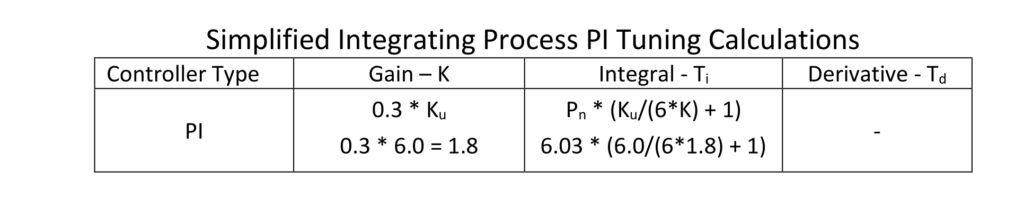
The new tuning constants are:

K = 1.8

T_i = 9.38 minutes/repeat

These calculations tend to confirm our belief that both controller gain and integral are too aggressive. Controller gain is considerably smaller and integral is slowed down quite a bit.

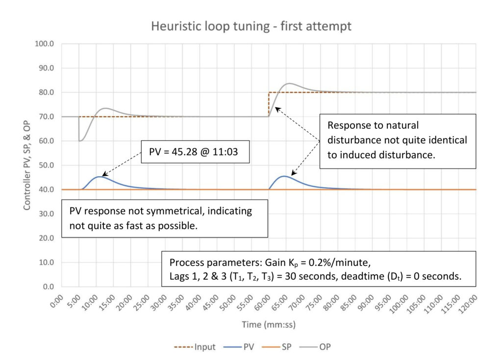
In Figure 4 we see that the new tuning constants are not quite as fast as possible based on the non-symmetrical response of the PV. The response to a natural disturbance is not quite identical, but is certainly close enough that we can have confidence that the tuning process will yield useful results. 

The easiest thing to do at this point is split the difference between the original and new tuning constants. The new estimated tuning constants are:

K = 2.9

T_i = 6.69 minutes/repeat

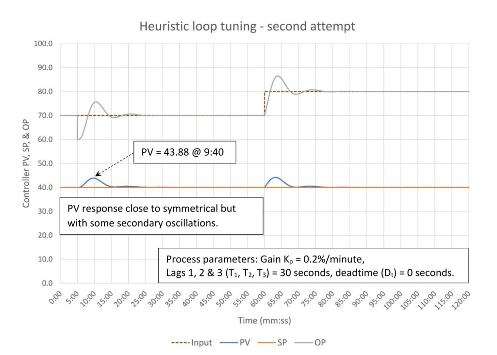
The process variable (PV) response in Figure 5 looks symmetrical but there are some mild secondary oscillations. The PV peaks earlier and at a lower value with these new tuning constants. If this were a noisy signal, we probably wouldn’t notice the oscillations.

Generally, at this point I would call it good and note the constants in the loop tuning log. But since we know there are multiple lags this may be a controller that might benefit from a little derivative. Integrating processes are not like self-limiting processes; you cannot set the derivative to one-fourth the integral and expect it to work. Instead, we should add a little bit of derivative at a time. In this case we will start with 0.25 minutes.

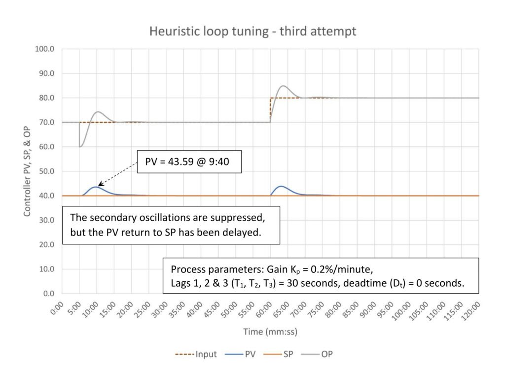
Figure 6 shows what happens when the derivative (T_d) is set at 0.25 minutes. Derivative penalizes PV movement, which means we should get a faster response when the PV starts moving resulting in a lower deviation from setpoint (SP). Adding derivative did indeed lower deviation from SP to 3.59 from 3.88, or about 7.5%. However, because derivative penalizes PV movement the PV’s return to SP is slowed down. If we were to continue to raise derivative the PV deviation from SP would continue to decrease (to 2.92 at T_d = 1.0), but the time for the PV to return to SP would continue to increase (to 15 minutes from about 8 minutes without derivative). This helps highlight the tradeoffs that are part of tuning integrating processes.

Example 2: Test of a controller mistuned for surge control

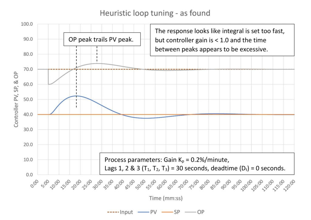
Figure 7 is the test of a controller mistuned for surge control. The visual cue, the controller output (OP) peaking some 9 minutes after the process variable (PV), indicates that the integral is tuned too fast. The normal response would be to slow down the integral, but with a controller gain below 1.0 we should strongly consider increasing the controller gain. We may still slow down the integral but the odds are if we do so the controller will not be capable of keeping the level inside the vessel should a large disturbance occur.

Before we retune this controller, we should decide what kind of performance we need from this controller. This is to be tuned for surge control, which means we need to pick how far we are willing to allow the PV to drift from setpoint (SP) and how fast we want to get the PV back on SP. I’m going to pick an arbitrary 30% PV drift from SP target and 60 minutes to return the PV to SP.

Because we were able to do an induced disturbance test, we can calculate the process deadtime and make an estimate of the process fill time from the process reaction curve. Note that the fill time estimate will be long because the controller is taking active measures to correct the process (the process gain will be low). In a worst-case scenario, the controller gain calculation could be oscillatory.

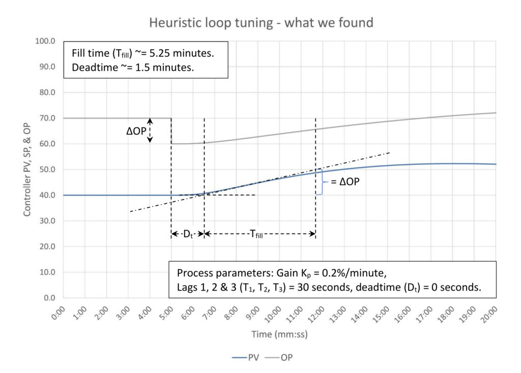
Figure 8 is a closeup of the initial process response. The standard open-loop tuning data collection method is used. A line is drawn through the steepest part of the response curve. Where it passes through the initial process variable (PV) determines the end of the deadtime. In this case since we are looking for the fill time, we pick the point on our line where the change in PV equals the change in controller output (OP).

Now that we have an estimate of the process deadtime and fill time we can calculate a controller gain using the open loop simplified integrating process PI tuning calculations from Table 1 in PID spotlight, part 14. Note that our estimated fill time (5.25 minutes) is longer than the actual fill time (5 minutes) by 5% (as expected). This shouldn’t significantly affect our calculations.

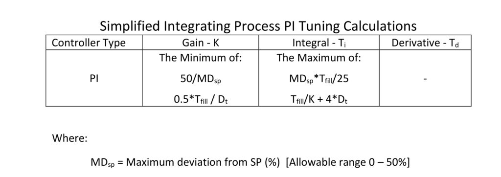
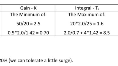
Based on a fill time of 5.25 minutes and deadtime of 1.5 minutes and our 30% deviation from setpoint allowance our tuning constant calculations are:

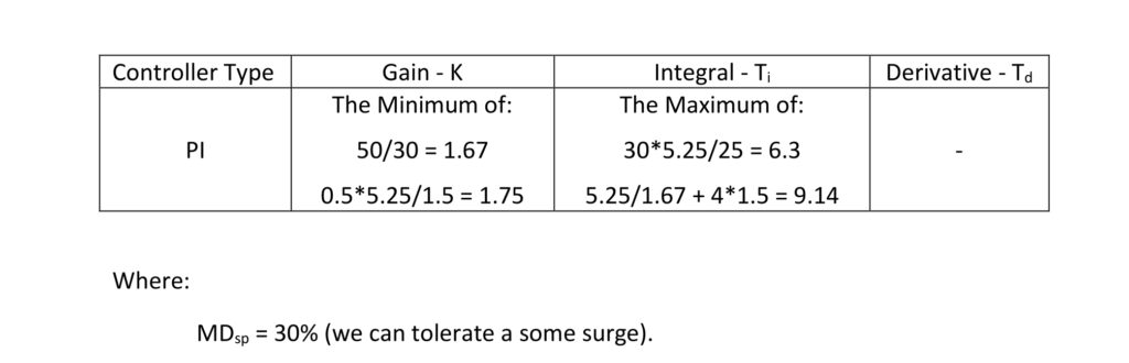
The new tuning constants are:

K = 1.67

T_i = 9.14 minutes/repeat

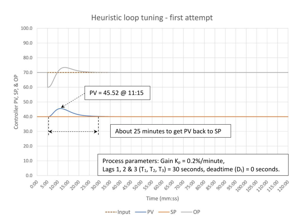
In Figure 9 we see that the PV deviation from SP is a little bit short of the targeted 60% of disturbance size (30/50) at 5.52%, but this is not unexpected given the presence of integral. The real issue is how fast the PV is returned to SP, ~25 minutes rather than the 60 minutes we specified. Doubling the integral to 18 will get us close (not shown).

Using shortcuts for level controller performance in the real world

I have used shortcuts here because they were available (and you should know they may be available). Unfortunately, unless you are actively working to optimize level controller performance you will likely only be called when a controller is performing poorly. You may walk up to a controller that is already swinging, however, using a shortcut requires that the process be at steady state so that you can execute a test.

When you cannot execute a test, you will be restricted to visual identification of the problem followed by increasing/decreasing gain and/or slowing down/speeding up integral. This may extend the time to resolve the problem. Because levels are slow, you should make a tuning change then walk away and do something else for couple of hours. Once you’ve stopped the continuous swing then you can work on optimizing controller performance.

Heuristic tuning tips

Heuristic tuning is generally safe since, except for the few seconds the controller will be in manual to execute an induced disturbance test (should you use this test method), the controller remains in auto. Regardless, work with the operator to determine the largest setpoint or controller output step the operator is comfortable with. Larger steps are preferred because noise and control valve problems will have less impact on the results. If you suspect that there are valve problems, you should make multiple steps of different sizes both up and down. If the process response is not the same, you likely have problems tuning cannot solve.

You should keep a loop-tuning log. There are a number of good reasons to keep a log; one is if you are using heuristic methods, you can use the log to guide your tuning efforts. Specifically, if you (for example) recently raised controller gain, and now it appears you went too far you can split the difference between the last setting and the current setting.

Heuristic tuning limits

Most integrating processes that we work with will be slow, and it is necessary for the response to play out fully to make accurate problem determinations. Of course, you can make rapid tuning changes if you walk up to a process that is performing poorly, and you can make an immediate problem diagnosis (this is why I like heuristics). Once you make that first change, exercise patience.

Heuristics can require multiple steps. If a control loop’s tuning is far off the mark it may be better to use open-loop tuning to get a first approximation and then use heuristics to finalize the tuning constants. However, if you are in a reasonably well-tuned facility and you find you must retune a control loop, it is very likely that the existing tuning constants are close to optimum. It will be far quicker to use heuristics, especially if there is a recent SP change in the trends, to estimate new tuning constants.

An induced disturbance test assumes that the process responds the same to input and output changes. If this is not substantially true, then the test results may not be valid.

A bad control valve will warp loop-tuning results. One of the more common problems with bad valves is hysteresis will induce a limit cycle swing. If you are not aware of the unique signature a bad valve creates, you may mistake this for a controller with too much controller gain or integral. Nothing you do will fix the swing, but your tuning efforts could slow the loop down to the point where it does not work.

Next steps: Bad valves and the mechanics of controller tuning

This concludes the discussion of tuning integrating processes. From here we will discuss some of the practical aspects of controller tuning beginning with how to spot bad control valves, how they affect controller tuning (it isn’t good) and what we can do about it (not much). Then we will discuss the mechanics of controller tuning. We will discuss how to figure out whether tuning is the real problem or if tuning will just cover up other problems. We will also discuss how to work with operators and how to avoid unsafe acts.

Ed Bullerdiek is a retired control engineer with 37 years of process control experience in petroleum refining and oil production. Send comments and questions to [email protected]. Edited by Mark T. Hoske, editor-in-chief,Control Engineering, WTWH Media, [email protected].

CONSIDER THIS

Open-loop, closed-loop and heuristic tuning methods are complimentary. How will having a working knowledge of the concepts behind all three methods speed and improve your tuning efforts?

ONLINE

PID series from Ed Bullerdiek, retired control engineer

Part 1: Three reasons to tune control loops: Safety, profit, energy efficiency

PID spotlight, part 2: Know these 13 terms, interactions

PID spotlight, part 3: How to select one of four process responses

PID spotlight, part 4: How to balance PID control for a self-limiting process

PID spotlight, part 5: What does good and bad controller tuning look like?

PID spotlight, part 6: Deadtime? How to boost controller performance anyway

PID spotlight, part 7: Open-loop tuning of a self-limiting process 

PID spotlight, part 8: Closed-loop tuning for self-limiting processes

PID spotlight, part 9: Heuristic tuning for a self-limiting process (part A on heuristic tuning)

PID spotlight, part 10: Heuristic tuning in a self-limiting process

PID spotlight, part 11: How a PID controller works with an integrating process

PID spotlight, part 12: What does good and bad controller tuning look like?

PID spotlight, part 13: Deadtime: what’s the best that I can do?

PID spotlight, part 14: How open loop tuning works in an integrating process

PID spotlight, part 15: Open loop tuning of near integrating processes

PID spotlight, part 16: Closed loop tuning of an integrating process 

Aug. 1 RCEP webcast available for one year: How to automate series: The mechanics of loop tuning

More on PID and advanced process control from Control Engineering.