PID, APC

 

A proportional-integral-derivative (PID) controller has limits and can be improved and optimized. Expansion of other control architectures doesn’t mean PID-based control systems are dying. Control systems are advancing with other technologies. Examples of control system advances follow.

Feed-forward control

Feed-forward control itself is another name for an open loop control. Such a control is not precise and cannot cope with the system disturbances, so it is very rarely used. However, it can be combined effectively with feedback control.

There are actually two options of the feed-forward combined with feedback control. They differ based on a variable, which is processed by the feed-forward path. Figure 1 shows both possibilities of feed-forward control (compensation).

Figure 1: A feedback control system can be enhanced with feed-forward compensation to enhance control system effectiveness. Courtesy: Peter Galan, a retired control software engineer

The first feed-forward compensation applies to a reference signal, r(t) with two blocks, F_y and F_u. The second feed-forward compensation applies to a disturbance signal, d(t). Such a feed-forward and feedback control arrangement is sometimes called a control system with disturbance measurement/compensation.

Feed-forward compensation

The first option under feed-forward compensation is explained below and shown in Figure 2.

Figure 2: A simplified block diagram combines feedback control and feed-forward compensation. Courtesy: Peter Galan, a retired control software engineer

In the simplified block diagram (Figure 2) the individual blocks represent transfer functions in the s-domain, omitting the s argument. The output-to-reference transfer function is expressed as

By choosing F_u = 1 and F_y = S, the response to the reference will be simplified to S, so it will not depend on C at all. This is great, as it’s possible to optimize control coefficients for minimizing disturbances, for example, without accounting for a response to the reference. However, the result is the same (slow) response time to the reference as the controlled system itself. In some cases, this does not matter, especially if the reference (set point) value rarely changes, or if such a slow reaction to the reference value change is even required. If this is not the case, then choose F_y to be a first order low-pass filter with a time constant, which can be, let’s say, 10 times shorter than the sum of the controlled system time constants. This is what the feedback control targets. Because F_y will not be identical to S, in this case a response to the reference value will remain dependent on the C parameters, but the sensitivity towards those control parameters/coefficients will be much lower, so it’s possible to optimize them to minimize the disturbance impact on the output variable. Usually, F_u and F_y are first-order filters (high-pass and low-pass respectively) with suitable time constants.

Disturbance compensation

A disturbance compensation is sometimes referred to as a feed-forward compensation applied to the disturbance signal. Look at the simplified block diagram of a combined, feed-back and disturbance compensation control system in Figure 3.

Figure 3: A simplified block diagram combines feedback control with disturbance compensation. Courtesy: Peter Galan, a retired control software engineer

The output-to-disturbance transfer function, in this case, is

By choosing F_d = S₁^-1, the output variable will not depend on a disturbance at all. However, such implementation is not as simple as it sounds. If S₁ represents a low-pass filter (which is almost always the case), the F_d should have the transfer function , which must contain a derivative. It’s even worse if S₁ contains some transportation delay. In such a case, F_d should be able to predict the disturbance behavior in advance.

That’s possible in some applications. For example, if the controlled system is a multi-zone heat chamber maintaining a certain temperature profile, current temperature can be measured at neighboring zones, and if they change, the control system can immediately act without waiting until they affect (disturb) this particular heat zone control.

Adaptive control

While feed-forward or disturbance compensations are more or less well-defined additions to a feedback control, adaptive control has rather a vague meaning. Basically, the purpose of an adaptive control is to monitor control system and its environment and modify either the structure, or more likely the parameters of a (PID) controller. Figure 4 shows a block diagram of a generic adaptive control system.

Figure 4: Block diagram shows an adaptive control system. Courtesy: Peter Galan, a retired control software engineer

Example: Adaptive control can work in a temperature control system that has continuously changing time constants of the heater. By analyzing the controlled system (the heater), it’s possible to measure its time response and calculate, for example, three pairs of its τ₁ and τ₂ constants, one taken at around the ambient temperature (τ^a₁,₂), the other one taken at the so called balanced temperature (τ^b₁,₂), at roughly 50% of the output power, and the last one taken close to the maximum temperature (τ^m₁,₂). Figure 5 shows those time responses are changing exponentially with the rising (falling) output variable: temperature.

Figure 5: Heater time response is graphed as a function of temperature. Courtesy: Peter Galan, a retired control software engineer

It’s possible to linearize time responses’ dependence on temperature, for example, as it is shown in Figure 6, which can simplify calculations provided by the adapter block.

Figure 6: Linearized time responses are graphed as a function of temperature. Courtesy: Peter Galan, a retired control software engineer

It is evident both time responses are functions of a difference between the actual temperature (an output variable) of the heating system and the ambient temperature. So, those two variables have to be inputs to the adapter block. Another information required by the adapter is the sign of actuating variable, u(t), because those time responses depend on whether the current process is heating or cooling. The adapter continuously calculates values of the controlled system time responses and calculates the optimal PID coefficients based on those values.

Optimal control

Optimally tuned PID parameters provide an optimal transfer function for a certain, reasonably selected time response (settling time) of an entire PID control system. However, the settling time, with which an output variable reacts to the step change of a reference value, even though it can be a “reasonable” short, it will not be automatically optimal, that is a shortest settling time possible. Further increasing the K₁ value may decrease the settling time. With continued increasing of the K₁ value, at some point the output variable will start to oscillate, which means the system is not optimally tuned and is unstable. To get optimal system behavior, for example, the fastest possible reaction to the reference value, a different control method is needed than a simple, closed-loop control system with PID compensation.

Optimal control has been a subject of extensive research for many decades, beyond the scope of this article, but below see some basic ideas about optimal control.

Example: A direct-current (dc) electrical servomechanism requires control. Such a servo system is very often used, for example in robotics. The servo requires control to reach a new reference point in the shortest possible time. An optimally tuned PID controller would not achieve this goal. Applying the maximum possible voltage to the dc motor runs the motor at full speed forward. At a certain time, changing voltage polarity, would start to de-accelerate the motor at the maximum possible rate. When the motor speed is zero, voltage is reduced to zero. By changing voltage polarity at the right time stops the servo at the desired position at the desired time. This is called optimal control, more specifically, time-optimal control.

Figure 7 explains the above-described time-optimal control process in the state space, which, in this case, is a two-dimensional space (area). One dimension is an output variable and the other dimension is its (time) derivative. At the moment, when a new reference value is applied, the output variable is shifted along horizontal axis, so it actually represents the regulation error – difference between the reference and the actual output. At the same time, t₀, a maximum voltage is applied to the dc motor. The servo leaves its initial position, P₀ and starts to accelerate. At the time t₁ the controller changes voltage polarity, and the motor speed decreases. At time t₂, just as the motor speed is zero and the desired position P₂ has been achieved, the actuating variable – voltage is turned off. While this seems straightforward, knowing the switching curve’s shape is not so simple.

Figure 7: Time optimal control in state space is graphed with derivative of output variable on the vertical axis, and output variable on horizontal axis. Courtesy: Peter Galan, a retired control software engineer

If the controlled system is a servomechanism with a simplified transfer function – the angular displacement over the voltage in the s-domain is:

where K and T include all the electro-mechanical constants of the servomechanism. A complete time optimal control system is shown in Figure 8.

Figure 8: Time optimal control system for servomechanism is shown. Courtesy: Peter Galan, a retired control software engineer

This is a different control scheme from PID control. It is non-linear control, and because the second non-linearity, N₂, represents a relay, such a control is called the bang-bang control. Regarding the non-linearity N₁, which represents the switching curve, the “sqrt” (square root) function will provide reasonable results. There are known graphical methods based on the isoclines

and some computational methods, which can be used to get a more precise switching curve. In practice, it is difficult, and the control process will likely be switching the driving voltage between its maximum and minimum forever. To avoid this, try to increase the dead zone of the relay. However, then the system may end up with a relatively high steady state error.

Another complication or limitation is the fact that not every controlled system exhibits “astatism” (meaning it contains an integral member) like a servomechanism. Such a system requires actuating the variable to be zero when the output variable matches the reference value. For example, a temperature control system maintaining certain temperature requires permanent presence of a non-zero value of the actuating variable.

In such cases, the time optimal control has to be combined, for example, with a feed-forward subsystem. The feed-forward will continuously provide some constant actuating value, which matches to a desired output value. The optimal control subsystem will act only as a booster during the transitions from one output value to the other.

An entirely different class of bang-bang control systems should be rather called on-off control systems. They are among the simplest systems, where the actuating variable changes its value between 0 and U_max forever. Their relay characteristics is a simple on/off with a small hysteresis in some cases. They are used in simple applications such as electric range heaters.  

Fuzzy control, a non-linear control method

Fuzzy controllers, a completely different alternative, are non-linear controllers. Fuzzy controllers belong to a class of artificial-intelligence (AI)-based control systems, which are becoming more popular. For example, in digital cameras almost every camera feature (like autofocus) is controlled using fuzzy-logic-based control systems.

A fuzzy control is another non-linear control method, which can be very good solution for such controlled systems, which are difficult to analyze, or their dynamic behavior is unknown at design time.

Examples: There’s a need to design a universal temperature control system for “any” type of heating system, or there’s a need to control a servomechanism with the variable load. In such cases the optimal PID coefficients cannot be found for a classical feed-back control, nor for the precise switching curve for the time-optimal control.

Fuzzy control can be compared to a “sub-optimal,” time-optimal control, that is, to time-optimal control, which can deliver worse-than-optimal results, though they can be still very good.

Fuzzy control can be seen as an extension or modification of fuzzy logic.

Three phases of fuzzy logic

The fuzzy logic, in the first phase, converts the “crisp” input variables into the “fuzzy” sets (in a process known as fuzzification).

Fuzzy logic, in the second phase, processes those fuzzy sets.

The final phase of fuzzy logic converts the processed fuzzy sets back to the crisp output variables (in a process known as defuzzification).

For the fuzzification of input variables, select, for example, a set of 5 “membership” functions of the lambda shape ( _/_ ). Estimate the entire range of input variables, which could be the same state variables, used in the optimal control (an output variable error and its derivative) and select 5 representative values. Those values, for example for the regulation error, could be -500, -250, 0, 250 and 500. They can represent the large-negative (LN), medium-negative (MN), small (S), medium-positive (MP) and large-positive (LP) levels. Each membership function will peak (reaching a value of 1.0) at the level, which it represents, for example the MN membership function peaks up at the regulation error value of -250 and acquires zero values for regulation error bellow -500 and above 0.

Similarly, define the membership functions for the second input variable.

During the fuzzification process, current values of the input variables will be converted to their membership function set values. For example, if the current value of a regulation error is 200, its membership functions (starting with LN up to LP) will acquire the following values: 0, 0, 0.2, 0.8, 0. Notice, the maximum two functions can acquire non-zero values and their sum has to be always one.

Processing the fuzzy sets is the most critical phase of the entire fuzzy control. It is “governed” by the “fuzzy control knowledge base.” How should such knowledge base be designed? The best approach is to use again the state space. A modified, two-dimensional state space (as Figure 7 shows), includes the fuzzified input and output variables, as Figure 9 shows.

Figure 9: In this fuzzy control knowledge base graph, first look at a representation of the input variables (the regulation error, err and its derivative, derr). Both input variables are shown as the “crisp” values and how they would be represented by a membership function sets. The main square is the entire state space. Courtesy: Peter Galan, a retired control software engineer

In Figure 9, first look at a representation of the input variables, the regulation error, err, and its derivative, derr. Both input variables are shown as the “crisp” values, as they would be represented by membership function sets. The main square is the entire state space. Its center (origin), clearly seen as a central part in Figure 7, in Figure 9 represented by the bold letter S in the small square in the center of a main square. The small squares represent levels of an output variable of the fuzzy controller, such as levels of an actuating variable, which drives a controlled system.

In the example, the output variable of a fuzzy controller can achieve, similarly like the input variables, 5 levels, so it can be represented by a set of the same membership functions, LN … LP. Of course, they correspond to different physical variables. For example, they can mean the driving voltage, -5, -2.5, 0, 2.5 and 5 V, respectively.

To create the knowledge base, the control designer must have an adequate knowledge of the control system behavior, usually based on feelings or rational observations, rather than on specific knowledge of time constants, gains and other physical attributes of the controlled system.

Fuzzy logic requires fuzzy rules

The fuzzy set processing means applying fuzzy rules. Fuzzy rules are typical production rules in a form:

< if … then … >

widely used in expert systems.

In this example, fuzzy rules will have a specific form, such as

<if (err == LP and derr == MN) then output = MP>

The “if” statements will have to evaluate each combination of the fuzzified input variables. Because there are two input variables, and each is decomposed into 5 states, 25 combinations of the input states exist, meaning there will be 25 fuzzy rules. Because up to 4 rules can have true value (remember, both input variables can be mapped to up to 2 membership functions), the question is what will be assigned to the output. This is a subject of the third phase, defuzzification.

Third phase: Defuzzification

The defuzzification is an opposite action to the fuzzification. Its purpose is to convert a level (actually several levels) of the fuzzy output variable to a single crisp value.  There are many ways to perform defuzzification, similarly like there are many ways to do fuzzification.  The most common method is called the “min-max” method. The min-max method selects only a maximum or minimum values from each fuzzy rule for further processing. Procedurally, the most convenient way to implement defuzzification with this method, is to combine it with fuzzy rules processing.

In a case when fuzzy rule (the “if” statement) consists of two or more conditions “ANDed” together, a minimal weighting coefficient (the fuzzified input variable with a minimal value) is selected as a combined “true” value for further processing. In fuzzy rules consisting of two or more conditions “ORed” together, a maximum weighting coefficient is selected for further processing. These rules are consistent with the theory of sets. The example uses only ANDed conditions, but different applications may use ORed conditions as well.

The following pseudo-code explains how the weighting coefficients and the output levels are processed in one fuzzy rule evaluation:

If the “if” expression above yields a true value (both ANDed values are true), the minimum value of weighting coefficients of both fuzzified input variables is assigned to an auxiliary variable, minV.  The minV value is added to another variable, den (denominator), and after multiplication with the mapping value corresponding to the produced output level, the product is added to another variable, num (numerator).

Figure 10: Defuzzified output variable is shown in a three-dimensional representation. Courtesy: Peter Galan, a retired control software engineer

These actions are repeated for each true “if” statement, for up to 4 statements, in the example. The num and den variables must be reset before being used in fuzzy rules processing. After the whole set of fuzzy rules is processed, the ratio num/den will yield a crisp value of the output variable. For example, if the current value of err is 200 and derr is 60, the resulting output value should be -1.428 (V).

The process described above is known as “singleton” defuzzification. The simplified “centroid” method got its name because of the resemblance to calculation of a center of mass of complex objects.

A surface containing values of the defuzzified output variable is called a “control surface,” because it determines the value of a control (actuating) variable for any given input values. In Figure 10, the surface represents a linear cut through a cube led symmetrically from one corner to the other. That’s expected because for this fuzzification, a set of linear and equally spaced membership functions has been used, and fuzzy rules do not exhibit any “irregularities” but yield constant output levels diagonally placed from the lowest to the highest. Mapping of the fuzzy output to its crisp values is linear also.

Of course, such a “flat” control surface is not the only output a fuzzy controller can deliver. The output can be made non-linear. At first, modify the membership function appearance. They do not need to be symmetrical, lambda-shaped functions. The only requirement is after the fuzzification of any input variable value, the sum has to be 1.0. Modify the knowledge base so its “switching curve” (a curve where the output variable changes its sign) will resemble a switching curve of the optimal controller, as Figure 11 shows.

Figure 11: Modified Knowledge Base can be modified to resemble Switching Curve (where the output variable changes its sign, resembling a switching curve of the optimal controller. Courtesy: Peter Galan, a retired control software engineer

Example: Try a different assignment of output levels to the output variable. This will change the shape of the output profile line as Figure 12 shows. It can be made similar to the N2 relay characteristics used in the optimal control.

Fuzzy control implementation, use

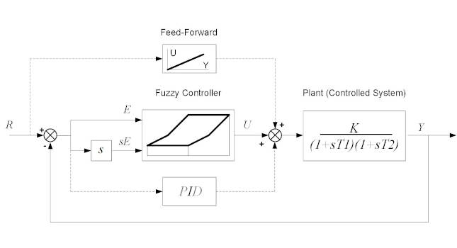
How might a fuzzy control be implemented? As it is based on the same state variables like the time-optimal controller, its block diagram will be very similar, as Figure 13 shows. Because the controlled system (plant) in the example is not an astatic type, when the output variable achieves its target value (i.e. being equivalent to a desired value, R and both, err and derr become zero), the fuzzy controller’s actuating variable, U, would become zero. But the controlled system requires applying such actuating variable, which would keep the desired output. And this is what would have to be provided, either as a feed-forward value, or as an output of a (collapsed) PID controller having just an integrator. Figure 13 shows a complete block diagram of a fuzzy control system.

Figure 12: Modified Shapes of Output Profile Line results from a different assignment of the output levels to the output variable. Courtesy: Peter Galan, a retired control software engineer

Similarity with the optimal controller is apparent. If the optimal controller in Figure 8 had to control the same plant like the one shown in Figure 13, the same requirements, for either a feed-forward or a collapsed PID controller would apply.

What is the difference, then, between those two control systems? An optimal controller requires knowledge of the controlled system parameters, especially its time constants. Without time constants, the switching curve would not calculate accurately. A fuzzy controller can “simulate” the optimal control performance, and, while results might not be as good, it will work with an entire class of a similar controlled systems without knowing anything about their dynamics.

Figure 13: Block diagram of a fuzzy control system is similar to the optimal controller. A fuzzy controller can “simulate” the optimal control performance, but while it might not achieve as good results, it will work with an entire class of a similar controlled systems without knowing anything about their dynamics. Courtesy: Peter Galan, a retired control software engineer

Beyond fuzzy controllers: Artificial neural networks

Is then, for example, a fuzzy controller at the peak of a control system theory and implementation? Yes and no. As mentioned, while fuzzy control is widely in many applications, including digital cameras, the industrial control applications are looking toward another, even more modern, technology, artificial neural networks (ANN). ANN-based controllers are even more complex than fuzzy-logic-based controllers, are deserve a dedicated article, which will be linked here when completed.

Peter Galan is a retired control software engineer. Edited by Mark T. Hoske, content manager, Control Engineering, CFE Media and Technology, mhoske@cfemedia.com.

MORE ANSWERS

KEYWORDS: Control methods, advanced process control, feed-forward control

CONSIDER THIS

If your control systems rely on decades-old control methods, are you getting decades-old results?