Control valve sizing data can often be estimated without direct measurement of pressure or flow.
Control valve sizing insights
- A process dilemma can complicate parameters for sizing control valves.
- Understand the pump curve to help assemble information needed for control valve sizing.
- When sizing control valves, complicating factors may include control design, inlet, outlet and pipe size.
When it comes to sizing control valves, the minimum and maximum flows and the pressure drops are critical information. But if that information isn’t readily available, it is still possible to size a control valve using a tape measure, a pump curve, and a little process knowledge.
A process dilemma: Parameters for sizing
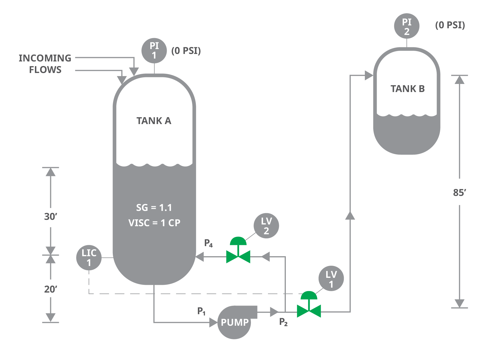
This process diagram (Figure 1) shows a common arrangement found in many process plants and facilities. Tank A receives varying incoming feeds from multiple sources, and a pump pulls fluid out of Tank A and sends it to Tank B. The level in Tank A is kept at setpoint by opening and closing control valve LV-1. Should LV-1 close fully, the pump would be deadheaded by operating against a closed valve, so a second control valve, LV-2, is added to open when LV-1 is mostly closed to keep the pump operating, with fluid flowing in the correct direction.
The task at hand is to size LV-1 and LV-2.
The key parameters for sizing a control valve include minimum, normal, and maximum flows; the inlet and outlet pressures; inlet temperature; and specific gravity of the fluid. The example shown in Figure 1 lacks the flow instrumentation typically used to gather this information, and it unfortunately mimics a large number of existing tank systems.
The two pressure readings (PI-1 and PI-2) are on the tanks themselves and may not be available for this calculation. The fluid characteristics are likely known; for this example, we will estimate it to be slightly heavier than water, giving it a specific gravity (SG) of 1.1, and with a viscosity close to water.
To get the rest of the information, we need to find the pump curve. That information can be obtained by checking the label on the pump and consulting the manufacturer. Most plants will have the pump curve on file as part of the pump documentation.
Understanding the pump curve
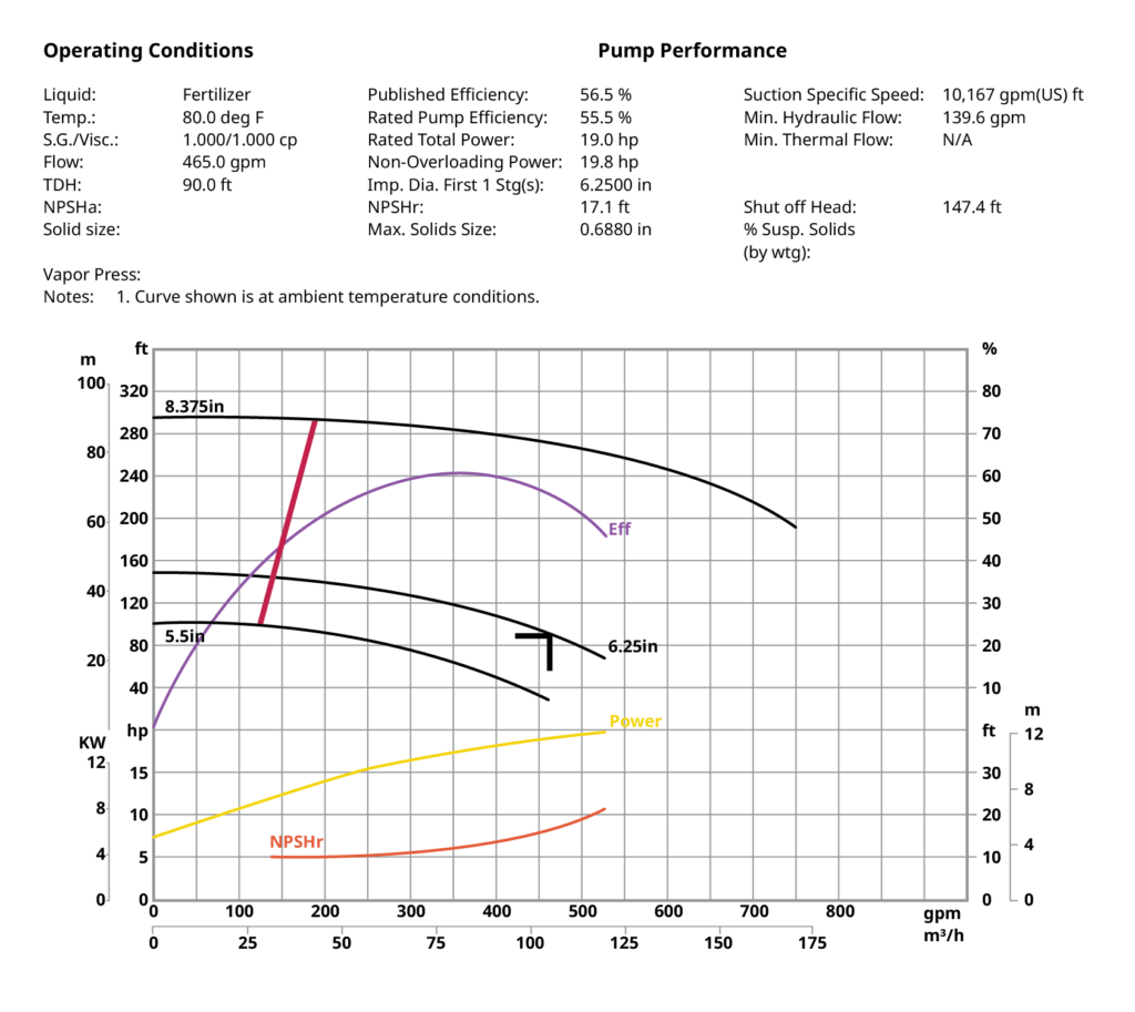
Pump curves come in different formats but generally look similar to Figure 2. Like control valves, pumps are specifically designed and specified to move a range of liquid flows at a specific range of differential pressures. Although pump curves can be daunting at first, they contain the missing pieces to the puzzle and can be relatively easy to read once the diagram layout becomes familiar, as explained below.
The three black lines in this particular curve show the flow in gallons per minute (GPM, X axis) versus the discharge pressure in feet of head (Y axis) for three different pump impeller sizes (5.5 inches, 6.25 inches, and 8.375 inches). The same pump may offer multiple impellers, with the larger impellers generating higher discharge pressures and more flow. In this case, the pump has a 6.25 inches impeller as indicated by the “Imp. Dia. First 1 Stg” in the description above the graph. The small triangle on the 6.25 inches curve indicates the design point of the pump, so this pump was sized to push about 465 GPM of flow at 90 feet of head.
The pump can operate anywhere on the curve, so it may move as much as 525 GPM, but at that flow the discharge pressure will drop to around 70 feet of head. The sloped red line indicates the minimum flow of the pump that is required to avoid cavitation and damage. This pump should not run less than about 140 GPM as indicated by the “Min. Hydraulic Flow” data at the top and the intersection of the red line and the pump curve. Based on this pump curve, we now know the minimum flow is about 140 GPM and the maximum flow is 525 GPM.
It may seem odd that a pump curve uses a strange unit like “feet of head” rather than a more standard unit like pounds per square inch (PSI), but that was done intentionally. Feet of head is an indication of the maximum height of liquid the pump can generate assuming 0 feet of head on the inlet. That height is not dependent on the specific gravity of liquid because the pump will generate the same number of feet whether the liquid is brine (SG=1.2), water (SG=1), or solvent (SG=0.7). All pump calculations are typically performed in feet of head to avoid complications of differing specific gravities. We will discuss how to convert feet to pressure in a later section, but for now we will investigate other aspects of the curve.
Most pump curves show other information, like the power required at various flow rates and the efficiency of the pump across the range of flows. Many curves also indicate a value called the required net positive suction head (NPSHr). This indicates the minimum pressure the pump needs at its inlet to operate without damage. If the pump operates below its NPSHr, it will tend to cavitate, move less flow, and ultimately damage the pump. This pump needs a range of 10 to 20 feet of suction head to avoid cavitation.
The pump curve assumes the suction pressure is 0 feet of head, but obviously the suction pressure will at least be equal to the NPSHr and will likely be higher than that. Therefore, the actual pump discharge head equals the suction head on the pump inlet plus the pump head shown on the pump curve. For this application, we have 50 feet of head on the pump suction, so when the pump is operating at the design operating point, the pump discharge head is (50 feet suction head) + (90 feet pump curve head) = 140 feet of discharge head at 465 GPM.
To determine the operating inlet and exit pressures of the pump, we will need to convert feet of head to pressure using the following equation:
(Feet of Head) x (SG of liquid) / 2.31 = Pounds per Square inch (PSI)
With that last piece of information, we are ready to determine the process conditions and size the valves.
Putting the information together for control valve sizing
To size a control valve, we need inlet and outlet pressures, and the expected range of flows. Unfortunately, our process diagram shows only the overhead pressure of both tanks (0 PSI each) and no flows at all. However, our pump curve has already provided the minimum, normal, and average flow rates of the LV-1 valve, and we know we need to at least flow 140 GPM or more through recycle valve LV-2 to avoid low flow pump damage. Now we need to determine the inlet pressure of each valve (P2), as well as the outlet pressures (P3) for LV-1 and (P4) for LV-2.
Fortunately, the pump curve tells what the pump head will be at a variety of flow rates, so one only needs to add the suction head (P1) to determine the pump discharge head, which can be converted to PSI to determine P2. If Tank A has no pressure on it (PI-1 = 0 PSI) and the suction pipe is short and sized correctly, then the suction head pressure for the pump equals 30 feet tank level plus 20 feet of additional pipe head for a total of 50 feet. Using our pump curve, we can now determine pump discharge pressure (P2) for a variety of conditions.
- At minimum flow (140 GPM), the pump discharge head is (50 feet + 145 feet) = 195 feet, and 195 feet * 1.1 / 2.31 = 92.8 PSI.
- At normal flow (465 GPM), the pump discharge head is (50 feet + 90 feet) = 140 feet, and 140 feet * 1.1 / 2.31 = 66.7 PSI.
- At maximum flow (525 GPM), the pump discharge head is (50 feet + 70 feet) = 120 feet, and 120 feet * 1.1 / 2.31 = 57.1 PSI.
Assuming the lines are short, the outlet pressure of the recycle valve LV-2 will equal the head pressure in the tank at that point converted to PSI. So P4 equals 30 feet * 1.1 / 2.31 = 14.3 PSI.
The pressure on the outlet of LV-1 (P3) will be the total of the liquid head plus the line pressure losses as the flow moves through that pipe. The head pressure is constant and equals 85 feet * 1.1 / 2.31 = 40.5 PSI. The line losses will vary with flow and can be calculated directly, but if the lines are not long and are sized accurately, the pressure drop is probably around 5 PSI or less per 100′ at full flow. Assuming our pipe is around 100′, the pressure at P3 equals 40.5 PSI + 5 PSI, which equals 45.5 PSI.
Sizing the valves
Despite an apparent lack of data regarding process conditions, we now have all the information necessary to accurately size both valves. To protect the pump from damage, the control system will open the LV-2 recycle valve to 100% when LV-1 is less than 10% open and close it otherwise.
Valve sizing information for LV-1:
• Liquid: SG = 1.1, Viscosity = 1.
- Minimum flow will be 0 GPM. At this condition, the inlet pressure is 92.8 PSI and the outlet pressure will be 40.5 PSI, so the valve must close against a maximum differential pressure (DP) of (92.8 – 40.5) = 52.3 PSI.
- Normal flow will be 465 GPM. At this condition, the inlet pressure is 66.7 PSI and the outlet pressure will be 45.5 PSI, so the valve is operating with a DP of (66.7 – 45.5) = 21.2 PSI.
- Maximum flow will be 525 GPM. At this condition, the inlet pressure is 57.1 PSI and the outlet pressure will be 45.5 PSI, so the valve is operating with a DP of (57.1 – 45.5) = 11.6 PSI.
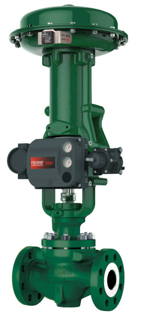
- Given the arrangement, an equal percentage valve will be a good choice because it provides acceptable low flow turndown, and high capacity at the upper end (Figure 3).
Valve sizing information for LV-2:
- Liquid: SG = 1.1, Viscosity = 1.
- Minimum flow will be 0 GPM. At this condition, the inlet pressure is 92.8 PSI and the outlet. pressure will be 14.3 PSI, so the valve must close against a max DP of (92.8 – 14.3) = 78.5 PSI.
- The valve needs to pass at least 140 GPM when open to avoid damaging the pump. Oversizing this valve will needlessly waste energy, so the max flow should probably be around 150 GPM to make sure there is adequate flow at 100% open, but not too much flow. The sizing conditions at 100% open are inlet pressure of 92.8 PSI and outlet pressure of 14.3 PSI, so the valve is operating with a DP of (92.8 – 14.3) = 78.5 PSI.
- Given the operating conditions, a linear, anti-cavitation trim will be a good choice for this valve, with the appropriate class rating for shutoff.
Complicating factors: Design, inlet, outlet, pipe size
This exercise is a simplified example, using a common control system design. Split range control isn’t the focus of this article, but the control system design is an important factor in successful operation of a system like the one in the example.
Furthermore, in a detailed analysis one needs to evaluate the inlet and outlet piping to determine the head loss as the liquid moves through the pipe. If the pipe is sized correctly, these values will be relatively small. But if the pipe is undersized, long, or has many bends—or if the liquid is viscous—these pressure drops can be significant and reduce the pressure drop available across the control valve.
The tank pressure may also come into play. For instance, if Tank A has 10 PSI of pressure in the vapor space, that 10 PSI would be added to the pump suction pressure (P1), the pump discharge pressure (P2), and the outlet pressure of LV-2 (P4). Similarly, five PSI in the top of Tank B would increase the LV-2 discharge pressure (P3) by five PSI.
Exact values for all these process values can be very accurately determined via an exhaustive piping system analysis, and if that information is available, it should be used. However, if no data is readily available and the plant lacks the capability to perform a detailed pipe calculation, it is usually possible to obtain reasonably accurate valve sizing information using a pump curve and a basic understanding of the piping system geometry.
Mark Nord is the control valve solution architect for Emerson’s flow controls products. Edited by Mark T. Hoske, editor-in-chief, Control Engineering, Arrowfly, [email protected].
Keywords
Control valve sizing, control valves, pump curves
Consider this
Are you sizing control valves correctly for your application?
You also might like