Sticking control valves warp loop-tuning results. Is that a nuisance or a potential disaster? Which way does a sticking valve warp the results and can we compensate? See three things about loop tuning with a sticking control valve.
Insights about tuning with sticking control valves
- Sticking control valves do warp open, closed and relay loop tuning results, causing all to overestimate controller gain. This can result in unstable tuning. Closed loop tuning will also cause integral to be slow. If you choose to use these methods anyway use a lower controller gain than the one calculated.
- Heuristic tuning is more resilient to sticking control valves. Tolerable results can be achieved with low risk if care is taken.
- You can test for a sticking control valve when performing open, closed or relay tuning.
- To spot a sticking valve during heuristic tuning you must recognize how a sticking valve affects controller response. There is not a separate test.
We are going to explore the claim “bad control valves will warp loop tuning results.” Just exactly how bad will it be? Can we still use the data from a test to estimate tuning constants, perhaps shading them in one direction to compensate for the error we know a sticking valve will induce in the loop tuning method?
How a sticking valve affects open loop tuning
In PID spotlight part 18, we discussed the importance of performing multiple steps when doing open loop tuning to identify whether the valve is sticking. In Figure 8 we saw that we could get wildly different results depending on the order of the step. We also discussed why it is important to make the biggest step possible.
So what happens if you ignore all this advice?

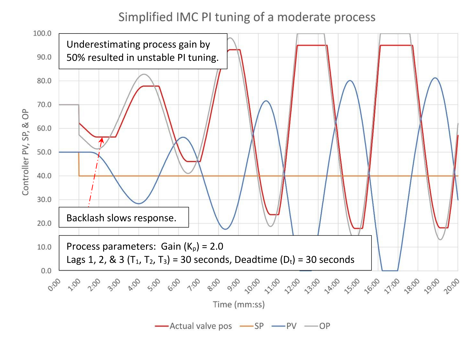
Figure 1 is the step test of the moderate self-limiting process. This is the same process used in PID spotlight part 7. In this case, however, the control valve sticks 5% with no slip. The actual valve position will trail the commanded position by 5% as long as the commanded position moves in one direction. Valve backlash is 10%.
In this particular step test, the actual position of the valve matched the commanded position at the start of the test. Because the valve only moved 5% our estimate of the process gain (Kp) is going to be off by 50% (1.0 estimated versus 2.0 actual). In reality our estimated process gain could have been anywhere between 0 and 2.0 depending on the actual valve starting position. Note that estimated deadtime and lag will still be close (there may be some additional deadtime as pressure builds in the actuator, but this is rarely more than a few seconds).
The change in estimated process gain will result in a controller gain of 1.26 versus 0.63 using the simplified IMC calculation method.

We can see in Figure 2 that underestimating process gain results in unstable control with proportional-integral control. You should note that the backlash of a sticking valve slows controller response when the process variable (PV) changes direction. This creates additional deadtime in the system that cannot be measured during an open loop step test. Of course, we know that adding deadtime to the process lowers the controller gain stability limit. We get caught in a double bind; underestimated process gain causes us to overestimate controller gain and the sticking valve creates deadtime that lowers the maximum controller gain we can use.

In Figure 3 we see that adding derivative per the simplified IMC tuning rules stabilizes the controller. The derivative is speeding up the controller output (OP) movement enough to shorten the apparent deadtime to the point that the controller is barely stable. We can also see that by the second oscillation the classic shark fin shape starts to appear in the process variable (PV).
In summary, the worst-case scenario of our failure to check for a sticking valve is unstable controller tuning. That said, if you suspect the control valve might be sticking testing the valve should help you identify if there is a problem and also allow you to get a more accurate estimate if you do a down-up-up (or up-down-down) test. You might also consider using a controller gain that is smaller than estimated, especially if the new controller gain is much larger than the existing controller gain, as a large change may be an indicator that the test results are suspect.
How a sticking valve affects closed loop tuning
The closed-loop tuning method provides an opportunity to test for a sticking control valve. Starting a continuous swing involves either changing the controller setpoint or stepping the controller output and then placing the controller in auto. If either method fails to start a swing, then the control valve is sticking. Taking progressively bigger steps will allow you to estimate the control valve backlash.

In Figure 4 the progressive stepping of the controller setpoint (SP) doesn’t elicit any process variable (PV) movement until the 6-minute mark. After we stop stepping the SP, we can see based on the final turn of the PV that there is about 1 minute of deadtime, so we can say that the 10% move at the 5-minute mark is what finally got us some kind of valve movement. Based on this, we can estimate the controller backlash is between 8% and 10%. (The actual valve position is trended so you can see what happens; this trend is likely not available on the control system.)
What happens if we do a closed-loop test anyway?

Figure 5 is a closed-loop test of the same process we tested in PID spotlight part 8 in Figure 1. With a properly operating valve the ultimate gain (Ku) was 1.26, and the natural period (Pn) was 3.42 minutes. A sticking valve causes the actual valve position to swing less than the commanded position, which creates the impression that the ultimate gain is higher, and the natural period is longer. One of the interesting things that showed up in testing is that the size of the initiating setpoint change affected the ultimate gain and natural period (see Table 1).

As the initiating setpoint step size increases, the estimated ultimate gain and natural period get closer to the actual process ultimate gain and natural period. Clearly bigger is better, but this is limited by how big a disturbance the process can tolerate.
Without the trend of the actual valve position, there is nothing in the closed-loop test that might warn us there is a problem with the test. The fact that there is a problem will become very apparent when we apply the new tuning constants.

Compare Figure 6 to PID spotlight part 8 Figure 3. Despite a higher controller gain and derivative the controller response is grossly inadequate. The response to the setpoint (SP) change is very sluggish because the actual valve position doesn’t respond very much to the initial output (OP) step. The integral is slower because the natural period was artificially lengthened by the control valve backlash. The response to the disturbance is very slow, exacerbated by the three minutes of additional deadtime caused by control valve backlash. The very obvious difference in deadtime between the setpoint response (1 minute) and the disturbance provides a visual cue that there is a control valve problem.
While it is not shown in Figure 6 if the control valve had started 5% behind the commanded position when the setpoint was changed the higher controller gain would have resulted in an oscillatory response as the valve moved a full 7%. This points to another visual cue that there is a control valve sticking problem, inconsistent response to setpoint changes.
How a sticking valve affects relay tuning
Relay tuning also will give us an opportunity to identify a sticking valve. If the selected control valve step size is too small, the process variable will not move, and the test will not happen (if you are running an automated test.) Similar to closed-loop testing you can take larger steps until you can induce a swing, however, if you cannot take a step size much bigger than the control valve backlash, then you should not use relay tuning.
But if you do anyway, see Figure 7.
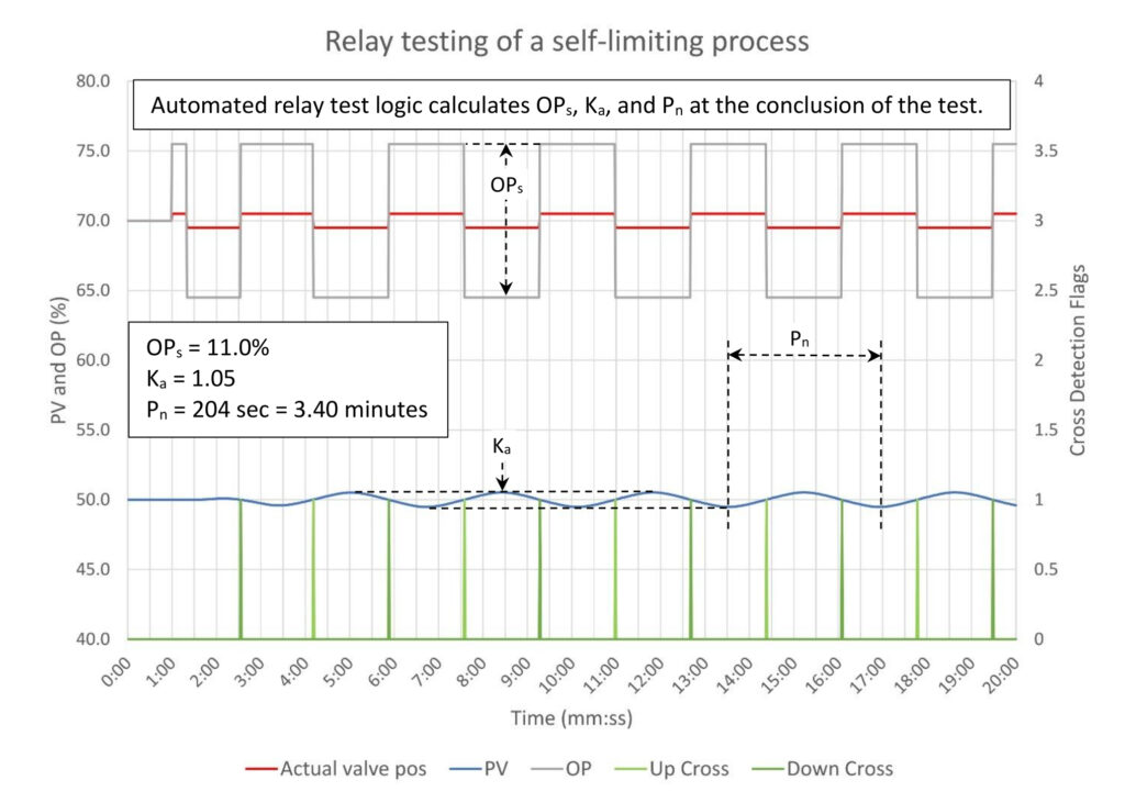
The vertical lines across the bottom of Figure 7 are when the software detects a SP crossing.
When we compare the results from Figure 7 with the results from PID spotlight part 8 Figure 4, we see a huge difference as explained in Table 2.

In Table 2 the calculated ultimate gain (Ku) from the relay test of the sticking valve is 11 times the value of the ultimate gain calculated for this process in PID spotlight part 8. The tuning constants calculated from these results will be wildly unstable. This shouldn’t be a surprise. In Figure 7 we can see that the actual valve position only moves 1% while the calculations assume the valve moved 11%, which readily explains the 11:1 difference in the ultimate gain calculation.
In short, if you suspect the control valve sticks very much, don’t use relay tuning.
How a sticking valve affects heuristic tuning
Heuristic tuning is based on pattern recognition and, unfortunately, we can expect a bad control valve to mangle the patterns we are looking for. Is all lost, or can we still manage to make some progress despite the problems?
To explore how heuristic tuning works when the control valve sticks we are going to work through the example from PID spotlight 9 starting with Figure 4.
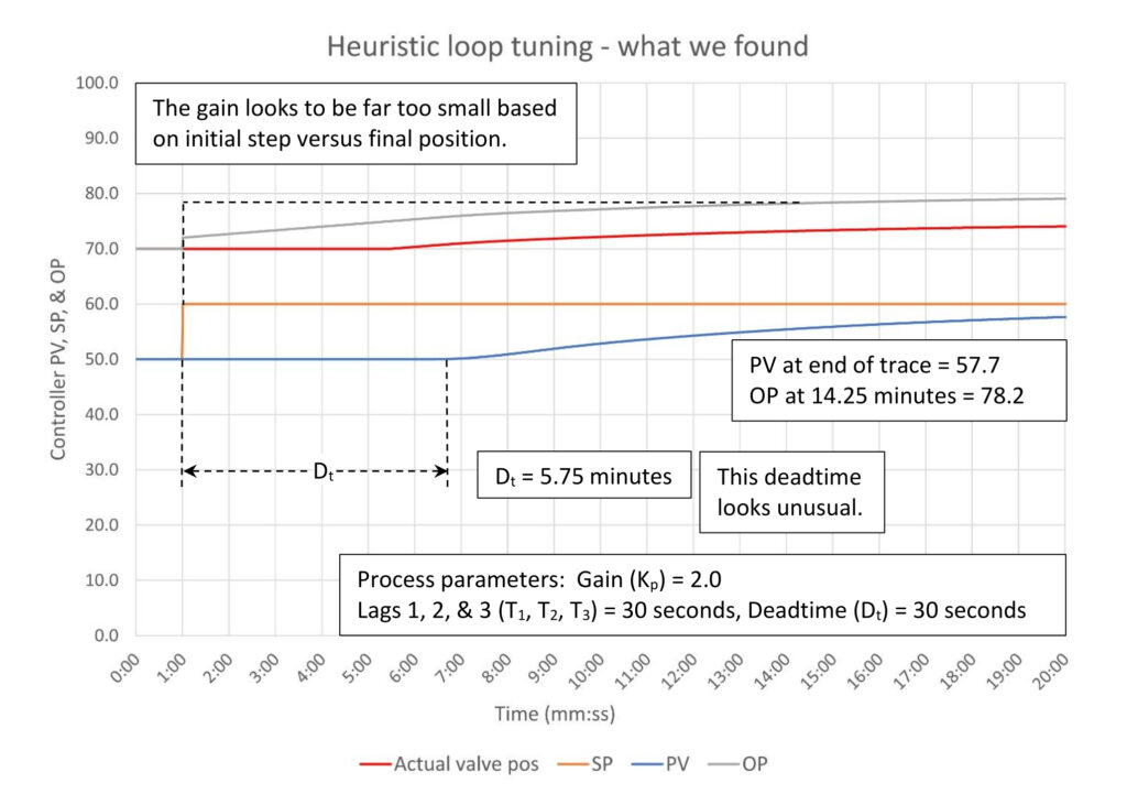
Figure 8 is the picture of a controller that appears to be tuned way too slow. The key parameters we want to pick off the trace are:
Deadtime = 5.75 minutes.
Kbase = (78.2 – 70)/(57.7 – 50)
Kbase = 1.06 (approximately)
I picked the controller output (OP) at 14.25 minutes versus 20 minutes for the process variable (PV) to compensate for the apparent deadtime. (Of course, what I don’t know at this time is the actual valve position is 73.2, and that most of the apparent deadtime is caused by backlash.)
Our best assessment is that the controller doesn’t have enough controller gain. The nearly six minutes of deadtime looks unusual, but there is no evidence at this point that this is a deadtime-dominant process. Nor is there any evidence that the integral tuning is a problem, so our first adjustment will be to increase controller gain. Normally the first adjustment to controller gain would be to set it equal to the baseline gain (Kbase), but in deference to the long deadtime and the possibility that this may be a deadtime dominant process, let’s split the difference and set the controller gain to 0.6.

More on the example: Deadtime dropped to under a minute
The first thing that jumps out at us from Figure 9 is the deadtime has dropped to under a minute. This is clear evidence that we have a control valve issue. If we look back at Figure 8 at the controller output one minute before the process variable started to move it looks like the output had moved about 5% from its starting point. Our guess is that this is the time when the valve actually started moving, and that this tells us that backlash is no less than 5%; it might be more. (But if our control system trended the actual valve position like this simulation does, it would be a lot easier to spot a sticking valve.) At this point I would manually step the controller output to determine how badly the valve is sticking.
Based on the final values of the process variable and controller output, it appears that the process gain (Kp) is about 1.0, however since we know that the actual valve position is now trailing the controller output by 5%, the process gain may be as high as 2.0, and therefore the baseline controller gain (Kbase) is likely closer to 0.5. This suggests that we might leave the controller gain alone for now.
However, we can see from the halting approach of the process variable to setpoint that the integral is far too slow. Let’s cut the integral 33% to 2.0 minutes/repeat.

In Figure 10 the first setpoint change results in what looks like a near critically damped approach to setpoint. However, the second setpoint change results in considerable overshoot. What’s more interesting is the controller output ends up lower after the second setpoint change than it was after the first. The controller output has worked through a considerable backlash induced deadband to return the process variable to setpoint. It’s obvious that this control valve has a significant sticking problem.
At this point I would ask the operator his preference between slower or faster swings. Depending on the downstream process either option might be preferable. If the operator doesn’t have an opinion, I would stop here, enter a maintenance work order to get the valve repaired and update the loop-tuning log.
In the end, the tuning constants we arrived at using heuristics with a sticking valve were similar to the tuning constants when the valve is good (see Table 3). In this case we got to tolerable tuning constants in two steps. It wouldn’t be unusual to require more steps, but in general we would use fewer steps because there is no need to optimize the tuning. The controller performance is going to be poor no matter what we do.

Heuristic methods are likely to get you to tolerable tuning constants when there is a bad control valve. It is still possible to have a very bad outcome if you are not properly skeptical. However, with proper care a bad outcome is unlikely.
Summary: Three things about loop tuning with a sticking control valve
A sticking control valve will warp loop tuning results. Please remember:
1. If the control valve sticks bad enough it is possible to calculate unstable tuning constants using open, closed, and relay tuning methods. All three methods will tend to calculate controller gains that are too big. Closed-loop tuning also will result in setting integral too slow.
2. If you choose to use any of these methods and you know that the control valve sticks, you can reduce the calculated controller gain to attempt to get a useful controller response. Start conservatively and work your way up, especially if you have used relay tuning. Consider speeding up the integral if you used closed-loop tuning.
3. Heuristic tuning appears to be more resilient when a control valve sticks. This is not to say that you can’t have a bad result, but if sufficient care is taken better results are likely.
Ed Bullerdiek is a retired control engineer with 37 years of process control experience in petroleum refining and oil production. Send comments and questions to [email protected]. Edited by Mark T. Hoske, editor-in-chief, Control Engineering, WTWH Media, [email protected].
CONSIDER THIS
Our control valve has issues. Can we still tune this controller? What method is likely to work best? What’s the worst that could happen, and how might I avoid it?
Aug. 1 RCEP webcast is available for one year: How to automate series: The mechanics of loop tuning
PID series from Ed Bullerdiek, retired control engineer
Part 1: Three reasons to tune control loops: Safety, profit, energy efficiency
PID spotlight, part 2: Know these 13 terms, interactions
PID spotlight, part 3: How to select one of four process responses
PID spotlight, part 4: How to balance PID control for a self-limiting process
PID spotlight, part 5: What does good and bad controller tuning look like?
PID spotlight, part 6: Deadtime? How to boost controller performance anyway
PID spotlight, part 7: Open-loop tuning of a self-limiting process
PID spotlight, part 8: Closed-loop tuning for self-limiting processes
PID spotlight, part 9: Heuristic tuning for a self-limiting process (part A on heuristic tuning)
PID spotlight, part 10: Heuristic tuning in a self-limiting process
PID spotlight, part 11: How a PID controller works with an integrating process
PID spotlight, part 12: What does good and bad controller tuning look like?
PID spotlight, part 13: Deadtime: what’s the best that I can do?
PID spotlight, part 14: How open loop tuning works in an integrating process
PID spotlight, part 15: Open loop tuning of near integrating processes
PID spotlight, part 16: Close loop tuning of an integrating processes
PID spotlight, part 17: Heuristic tuning of an integrating processes
PID spotlight, part 18: Identifying control valve performance problems
PID spotlight, part 19: PID controller tuning best practices