Can we have a PID controller respond quickly to large disturbances and have a more relaxed response to smaller swings? Can our PID controller respond quickly to constraint violations while allowing movement away from the limit? Can we limit controller interaction while still maintaining control within limits?

Insights about PID gap control
- Setpoint gap control can shape controller tuning to respond aggressively to large disturbances and have a relaxed response for smaller disturbances or to respond aggressively only on one side of the setpoint in constraint control situations.
- Setpoint gap control may be stable when the controller gain is above maximum recommended levels, allowing room for error when tuning calculations may be uncertain.
- Setpoint gap control can help break controller interaction when multiple controllers with similar dynamics are close together.
There are two situations where we should consider shaping proportional-integral-derivative (PID) controller response to match process requirements:
- Frequent large disturbances
- Controller interaction.
In both cases setpoint (SP) gap action is used because the change in controller response must follow the controller setpoint.
Frequent large disturbances
The oil processing areas of a refinery rarely see large disturbances, and therefore each controller has one tuning goal, whether it is disturbance rejection, critically damped or some variation of slow optimization. These controllers are also generally easy to test, which gives us good confidence in our tuning results.
However, the stormwater, wastewater and flare systems must routinely handle large disturbances caused not just by weather or process events but by automated pump, blower or compressor starts and stops. As a result it is not unusual to have two controller tuning goals; somewhat relaxed for normal operations and very aggressive for the large disturbances that are going to occur. These systems are also often very difficult to step test; we have to implement aggressive controller tuning on little or very suspect information. This leaves us plenty of opportunity for poor results. Controller gap action provides us a way to achieve our multiple tuning goals and hedge our bets.
Controller interaction
Limiting controller interaction refers to situations where a controller’s output shouldn’t move when the process variable is close to setpoint so that the rest of the process around it can settle but should move if a larger disturbance occurs. Normally you will find these situations where the controller affects other controllers (one way interaction) or this controller “fights” another controller (two-way interaction). In either case keeping this controller exactly on setpoint is less important than not upsetting the controllers around it.
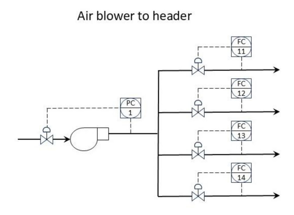
Figure 1 is a situation that is common in refining; a forced draft fan supplies air to (for example) a heater with multiple cells. Each cell has its own air flow controller, each of which is a secondary controller to a combustion control scheme (not shown). The individual air flow controllers are constantly moving following the combustion air flow requirements. Maintaining a constant blower discharge pressure (PC-1) will interact with the air flow controllers as they attempt to follow the setpoint changes from the combustion controls. This interaction can, in the worst-case scenario, result in safety system driven heater shutdowns.
We can take advantage of the fact that the air flow controllers do not require a specific header pressure to maintain flow. The pressure can be allowed to float a little bit. We can set an appropriate gap, which will allow the flow controllers to do their job without also having to “fight” the pressure controller. When the header pressure reaches a high or low limit PC-1 will nudge it back within the allowable range. (The flow controllers may still “fight” with each other; there are other methods that can help with this.)
In many processes there are situations where two controllers in series have similar dynamics. It could be a pressure and flow controller(s), as in this case, or some other combination. Keeping one of these controllers on setpoint will be more important than the other; consider using gap control on the less important controller to mitigate interaction.
Note also that interacting systems have complex dynamics. Depending on how bad the interaction is normal tuning rules may not apply. Using gap action on one controller may allow us to break the interaction enough that the more important (non-gapped) controller can be tuned using normal tuning methods and rules. The gapped controller will require more attention.
When can we use gap control?
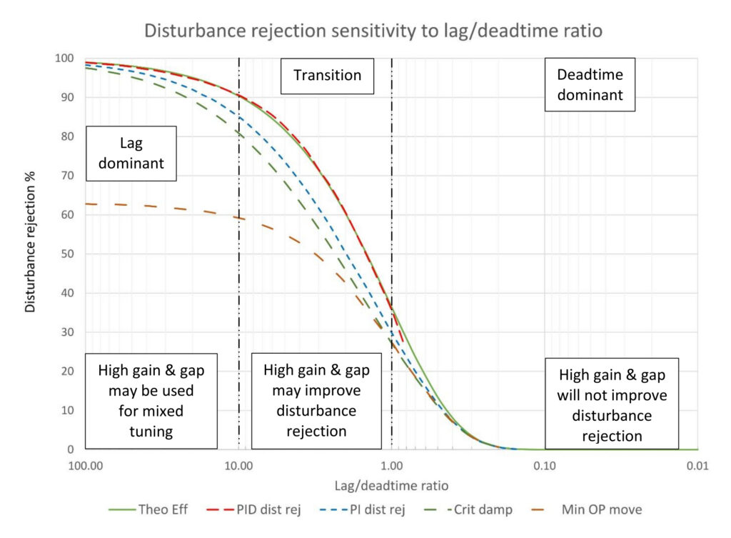
For gap control to be effective the process must be one where changing the controller gain affects disturbance rejection effectiveness. We’ve seen Figure 2 before (see PID spotlight, part 28 Figure 1; link to all prior articles in the series at the bottom), which maps disturbance rejection effectiveness across lag/deadtime (L/D) ratios from 100:1 to 1:100. There is a new green line (Theo Eff) which is the theoretical best disturbance reduction effectiveness that can be achieved on first order plus deadtime processes (FO+Dt). Some additional improvement is possible when a process has multiple lags, but it is limited.
Below an L/D ratio of about 1:1, PID controller tuning has little impact on disturbance rejection effectiveness, and below 1:5 disturbances are fully expressed and persistent (see PID spotlight, part 6). Using gap action here will only make control worse.
L/D ratios from 10:1 down to 1:1 are very sensitive to controller gain. If disturbance rejection tuning is required, an accurate measurement of the lag and deadtime, and therefore the L/D ratio, is necessary to be comfortable with the tuning. If you lack accurate measurements, aggressive tuning is risky.
Fortunately, controller gap action gives us an opportunity to hedge our bets. A sufficiently large low controller gain range, a gap, near the setpoint will allow a very aggressively tuned, perhaps even a normally unstable controller to stabilize after responding to a large disturbance. The tradeoff here is the gap will slow the initial response to a disturbance, which will lower the disturbance rejection effectiveness. Increasing controller gain outside the gap can help make up the difference, but the L/D ratio of the process sets an absolute upper limit on possible disturbance rejection effectiveness. Beyond a certain point, increasing controller gain (and adding derivative or speeding up integral) doesn’t help.
However, if we are in a situation where the controller should be tuned less aggressively for normal control and only be sped up for large disturbances, then we have an opportunity to apply gap action. This can apply to situations where aggressive control is required on both sides of the setpoint or in cases where aggressive control should be applied only on one side of the setpoint (constraint control).
Gap action can also be used on processes with high (>10:1) L/D ratios. Here the problem is less about disturbance rejection and stability limits than it is about excessive controller output response affecting other parts of the process.
Planning a staged process response
Planning begins with an open loop step test. The test results are used to determine whether gap control can be used and to calculate two sets of tuning constants; typically, PI disturbance rejection tuning for large disturbances and something between critically damped and minimum controller output movement tuning for inside the gap. If disturbance rejection is required on both sides of the setpoint then careful consideration of the gap size is required. If this is a constraint control situation (you only care about disturbances on one side of the setpoint) then the gap on the safe side of the setpoint can be infinite. Setting the gap size requires knowing something about the maximum size of the disturbances and the maximum gain required to manage these. Simulation can be very helpful for setting the final tuning parameters.
All of that sounds very complicated. Circumstances may make heuristics a better approach. Start by setting a base set of controller tuning constants that works for ordinary process disturbances. Pick a gap and start raising the gain outside the gap. Let that run until several disturbances have come through and decide whether there is too much controller gain or not enough. Repeat until satisfied. You may find you have to adjust gap size during the process and/or lower the gain inside the gap. Depending on how often large disturbances occur this may take weeks or months of calendar time to get to a “final” set of tuning constants, but you will get there (and that approach is perfectly acceptable).
If it hasn’t already been done, test the system to verify the PID algorithm and whether the system uses the positional or velocity PID algorithm form. The results will identify which gap algorithm can be used and if some gap algorithm customization may be required. The possibilities are:
- Classical algorithm, velocity form: Notch gap.
- Classical algorithm, positional form: V-notch, possibly customized for constrain control.
- Parallel algorithm, either form: Error squared, possibly customized for constrain control.
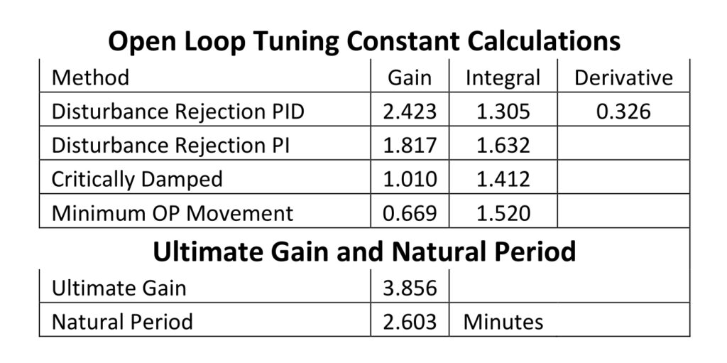
The following examples will use a process with a 2:1 lag/deadtime ratio to illustrate pushing controller tuning. The process parameters are a process gain of 1.0, three lags of 30 seconds and a deadtime of 13 seconds, which results in a lag of 87.7 seconds and deadtime of 43.3 seconds for a calculated L/D ratio of 2.03:1. Table 1 summarizes the calculated tuning constants, ultimate gain and natural period. (Real world data will never be this precise.)
Notch gap setup for a classical PID controller; velocity form
There is some art to setting up a SP gap application. Instead of one decision there are now three; two tuning performance targets and the gap size. Rough numbers will work, especially if the step test results are estimates. For large disturbance applications start with a disturbance rejection controller gain value; for this process that will be 2.4 (PID disturbance rejection from Table 1). The gain multiplier will be set to provide an effective controller gain inside the gap between minimum output movement and critically damped; in this case 0.3 (0.7/2.4). Integral should be set slower; 1.5 minutes/repeat is used based on minimum output movement tuning. The gap is set to cover the range of normal disturbances, typically ± 5 or 10%.
Don’t think too hard as these numbers will likely be changed once the educated guesses reach the real world. In this case the controller tuning was a bit oscillatory, and some derivative (0.1 minutes) was added to knock down the swings.
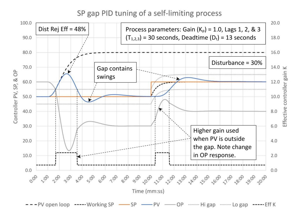
Figure 3 shows the results of the final controller tuning. It is very obvious when the controller gain changes by how the controller output (OP) response changes. When the process variable (PV) is outside the gap, the OP moves much more rapidly. This does result in PV overshoot, but this is contained inside the gap, which allows the controller to settle.
Disturbance rejection efficiency on the 30% disturbance is 48%. This is considerably less than the 65% reduction that could be achieved using PID disturbance rejection tuning. This is part of the tradeoff for using less aggressive control for “normal” operations and reserving aggressive responses for large disturbances. On the other hand, this is much better than the 39% disturbance rejection efficiency that minimum OP movement tuning would provide.
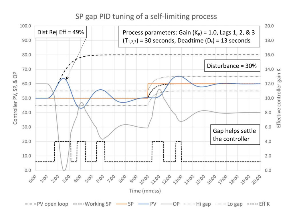
Figure 4 illustrates a benefit of using SP gap control; if the controller gain is very high the controller will still be stable (up to a point). The ultimate gain for this process is 3.8 (Table 1) but the controller gain is 4.0. Without the SP gap this controller would be wildly unstable. Note that the disturbance rejection effectiveness increases only 1% (49% versus 48%) despite the large increase in controller gain. Ultimately, the effectiveness of increasing controller gain to reduce disturbances runs up against theoretical limits and further increases have little or no effect.
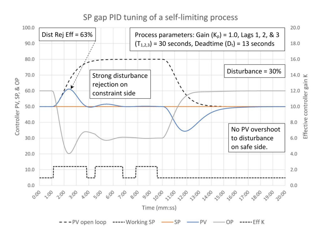
Figure 5 shows how gap control is used for constraint control. The tuning on the constraint side of the setpoint is set as aggressive as you dare, in this case for PID disturbance rejection. The gain multiplier is set to reduce controller aggressiveness to no more than critically damped. The gap on the constraint side of the setpoint is set very small (0.1%) and on the other side somewhere arbitrarily far away (30%). On the constraint side of setpoint, the response to a disturbance should minimize the PV movement from setpoint and return it to setpoint as rapidly as possible without oscillation; overshoot is not a concern. A disturbance that pushes the PV in the safe direction should avoid PV overshoot as it works to correct the disturbance. Disturbance rejection effectiveness, arrest and recovery time are less important on the safe side of the setpoint.
The disturbance rejection effectiveness on the constraint side is much better at 63% here because the small gap above the setpoint does not allow the PV to gain momentum before aggressive controller response begins. Compare this to the gap controller in Figure 3 (48%). If an application requires aggressive control of large disturbances on both sides of the setpoint but needs to be shaded on one side the gap limits could be offset to 0.1/10% instead of ±5%. This is still a 10% gap, but the PV will tend to run on the safer side of the setpoint.
V-notch gap setup for a classical PID controller; positional form
The V-notch gap calculation used in this example is:
K = ABS(Error)*Kslope/10 + Knotch
Where:
Kslope is how fast the controller gain should increase per 10% error.
Knotch is the controller gain when the error is zero.
The setup is a little different than the notch gap algorithm because you set the lower control gain and then set the slope calculation for the higher gain. The lower control gain can be zero, in which case the V-notch gap algorithm acts just like the error squared gap algorithm.
We are going to attempt to set this example up to act like the notch gap example above using critically damped tuning when the error is zero and disturbance rejection for a large (30%) disturbance. Setting Knotch is easy; it’s just the gain for critically damped tuning (rounded to 1.0). Integral can be 1.5 minutes/repeat.
Setting Kslope is a little more complicated. We would like to start with something that is safe and work from there. If we assume that the normal controller setpoint is 50%, and therefore the error can never be more than 50%, and that the controller gain should never be higher than the ultimate gain (Ku), then we can back-calculate a slope using:
Kslope = (Ku – Knotch)/5
In this case:
Kslope = (3.9 – 1.0)/5
Kslope = 0.58
This might be a bit conservative. From here we can increase the slope in increments until there is evidence of too much controller gain and then cut back (see PID spotlight, part 9 for heuristic tuning rules).
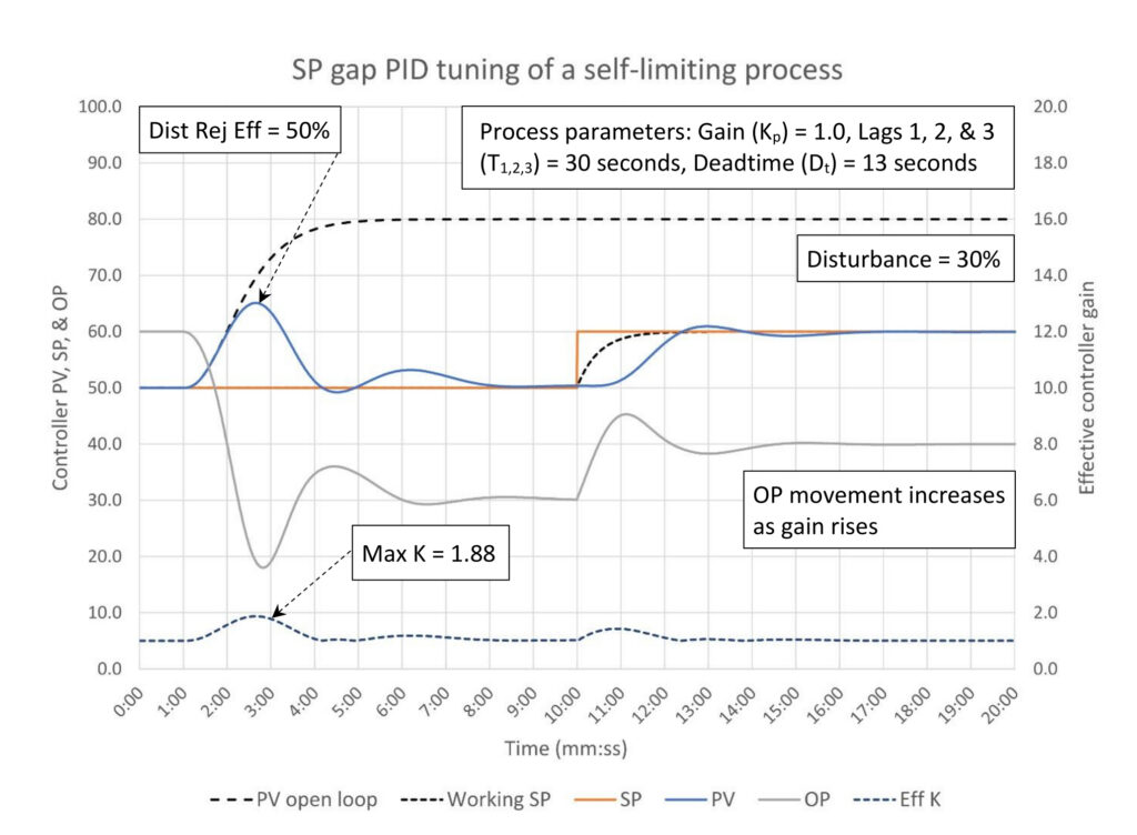
Figure 6 shows the response of the V-notch controller after some minor adjustments. As with the notch gap controller, some derivative had to be added to knock down oscillations. The maximum controller gain only reached 1.88 instead of the 2.4 we were targeting, but the disturbance rejection effectiveness is 50% versus 48% for the notch gap controller in Figure 3. Raising Kslope to 1.0 will cause the controller gain to match the 2.4 we were aiming for, but only increases disturbance rejection effectiveness to 52%. Furthermore, the controller response gets more oscillatory. Increasing derivative doesn’t help to reduce oscillation. Therefore, based on the (highly subjective) eyeball test, the tuning constants used here are about optimal.
Like the notch gap controller, the V-notch is somewhat tolerant of excessive Kslope or Knotch values. No figure is provided to demonstrate what happens, but the controller response will look like there is too much gain per heuristic tuning rules. Heuristic tuning rules can be used to correct the problem.
If constraint control is required, a custom V-notch gap algorithm must be programmed. At a minimum, a different Kslope can be programmed for either side of the setpoint. Additional enhancements could include a maximum controller gain and/or a flat gain area on either side of the setpoint. Naturally, more options further complicate tuning.
Error squared gap setup for a parallel PID controller
Any gap gain algorithm that works by calculating an error signal that gets passed to the PID controller has a fundamental limitation; the effective controller gain is zero when the error is zero. This produces a dead spot around the setpoint for the error squared and floating setpoint gap algorithms. The floating setpoint gap algorithm is not recommended for staged response tuning because it can only supply one style of tuning outside the gap and absolutely no response inside the gap. The error squared gap algorithm can be used if this limitation does not cause problems.
The error squared calculation used in this example is:
EPID = if(ABS(Eraw)>SD, Eraw, Eraw*ABS(Eraw)/SD)
Where:
EPID is the error signal fed to the PID controller (%)
Eraw is the calculated error (PV – SP) (%)
SD is the scaling divisor (%)
The operation of the error squared gap algorithm works just like the V-notch gap algorithm with the exceptions that the minimum notch gain (Knotch) is always zero and the maximum gain is the controller gain (K).
We are going to set this controller up to respond similar to the notch and V-notch gap examples above. We are looking for disturbance rejection tuning for large disturbances; let’s start with PID disturbance rejection tuning (K = 2.4, Ti = 1.3, Td = 0.33). Since we are looking at 30% as the benchmark for a large disturbance, setting the scaling divisor at 30% should be a good conservative starting point.
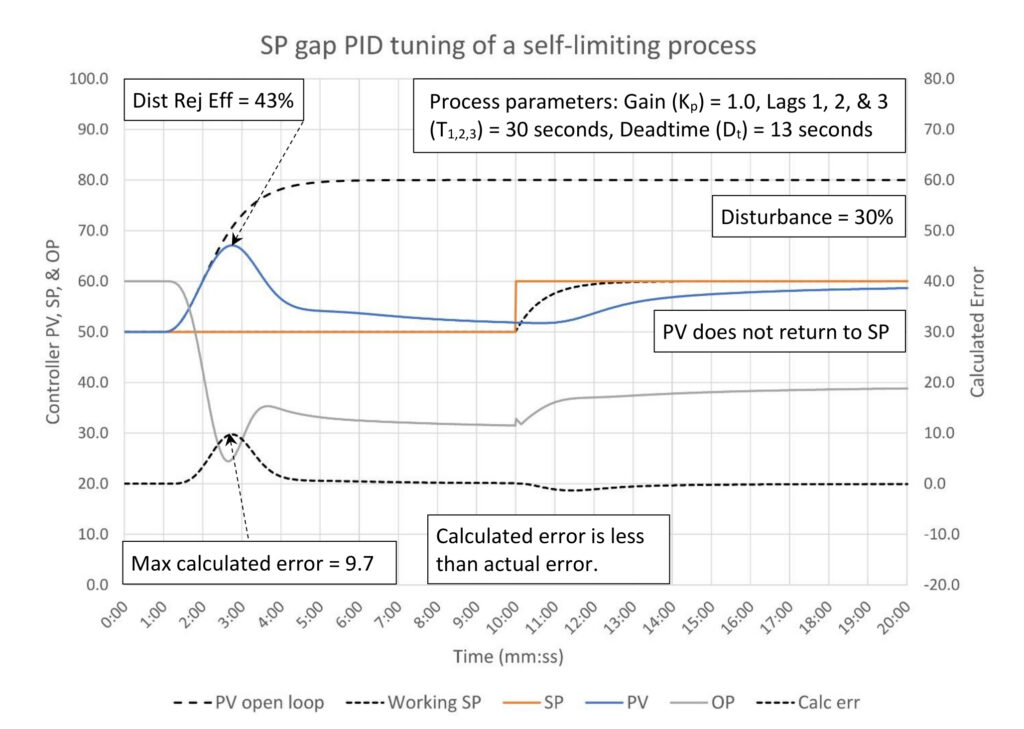
One problem with error squared gap control is shown in Figure 7; the process variable doesn’t come back to setpoint. When the calculated error that is passed to the PID controller drops close to zero there is no drive to push the PV back to SP. Another issue is because the effective controller gain starts at zero, the disturbance rejection isn’t as effective as the V-notch gap algorithm. The disturbance rejection effectiveness is only 43% instead of the 50% seen in Figure 6. To address this, we can look at reducing the size of the scaling divisor and/or increasing the controller gain.
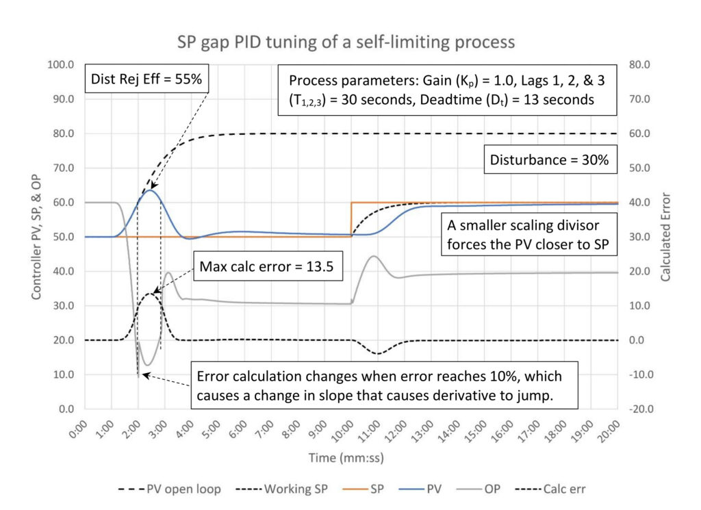
In Figure 8 the scaling divisor has been tightened to 10% and the controller gain raised to 2.6. This has considerably improved disturbance rejection effectiveness, raising it to 55%. It has also exposed a problem with using derivative with this gap algorithm. Once the PV moves more than 10% from SP, the error calculation changes from error squared to straight error. This creates a sudden change in direction in the signal passed to the controller, which causes derivative to spike. This is very apparent at the 2-minute mark where the controller output jumps up 10%. It is less apparent at 2:50 mark, but the controller output jumps 10% there also. This can be mitigated by using a derivative filter (if available). Also, the smaller gap created by the smaller scaling divisor improves the PV approach to setpoint.
Another option would be to increase the controller gain and widen the scaling divisor proportionate to the square of the change. The purpose of changing to straight error at the edge of the scaling divisor is to provide a safe maximum controller gain. We do know that the presence of a gap will allow controller gain to go as high as the ultimate controller gain and still remain stable. Taking the controller gain to 3.5 (close to the ultimate controller gain) should allow us to raise the scaling divisor to 20%.
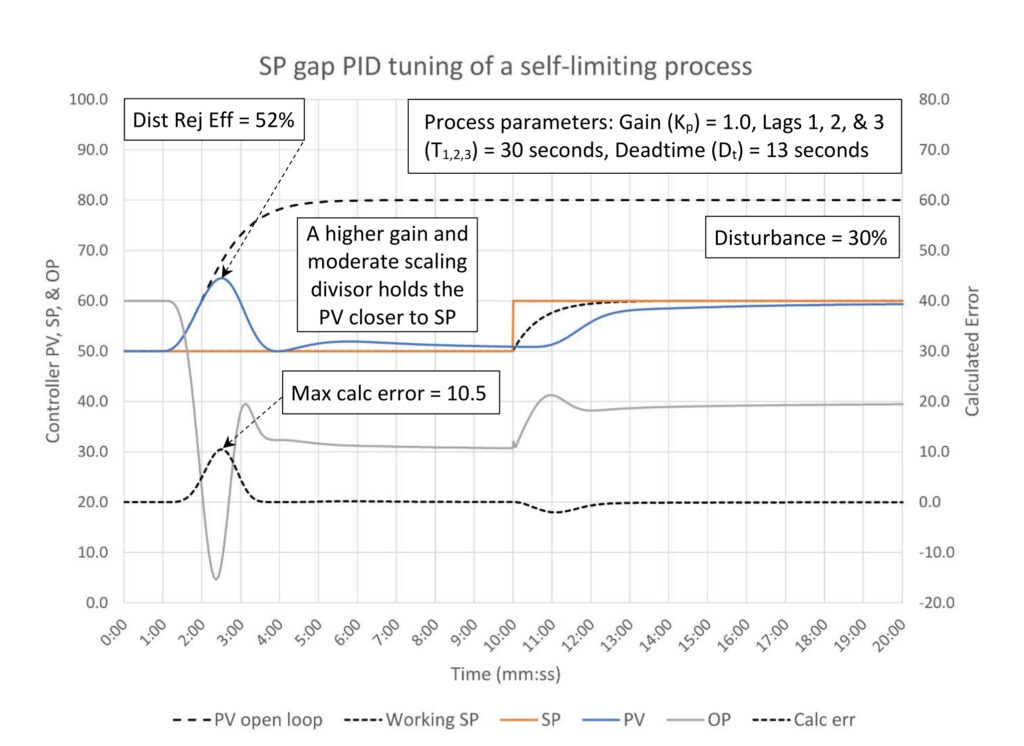
In Figure 9 it appears we have arrived at a reasonable tuning setup. Disturbance rejection effectiveness is a reasonable 52% for a process with a 2:1 lag/deadtime ratio. The disturbance is eliminated in a symmetrical curve, indicating gain and integral are well matched. The PV does drift off, and remains off, setpoint, but is better with the higher controller gain and smaller scaling divisor than the tuning in Figure 7. Otherwise the controller response is smooth with little oscillation.
Planning a gap controller to break controller interaction
Planning begins with identifying controllers that will interact and have similar dynamics. Then you must decide which controller(s) must stay on setpoint and which can be permitted to drift from setpoint. In the forced draft fan header example in Figure 1, the air flow controllers FC-11 through FC-14, being cascade secondaries, cannot allow air flow to drift. PC-1 has similar dynamics to the flow controllers and will, if tuned tightly, interact with the flow controllers. PC-1 could be detuned to limit the scope of interaction, but this also reduces the controller’s ability to react to disturbances. Gap action and appropriate controller tuning allows breaking interaction while maintaining reasonable response to disturbances.
Once we’ve decided which controller will be gapped, we need to decide how big the gap will be. For PC-1 the minimum will be somewhere above the minimum pressure to keep the flow controller valves within operating range, and the maximum will be somewhere below the blower’s maximum discharge pressure. In reality the gap limits likely can be well within those limits; they just need to be wide enough to prevent excessive valve movement.
The controller gain inside the gap should be zero, which limits our choices to the notch gain gap algorithm or the floating setpoint algorithm. The V-notch algorithm could be used after customization to supply a zero gain flat spot.
The following examples will use a process with a 2.1:1 lag/deadtime ratio, which is similar to a typical pressure controller in this process. The process parameters are a process gain of 1.0, lag of 10 seconds, a lag of 5 seconds and a deadtime of 5 seconds, which results in an apparent lag of 13.5 seconds and deadtime of 6.5 seconds. These dynamics are very similar to typical flow controller dynamics. Table 2 summarizes the calculated tuning constants, ultimate gain and natural period.
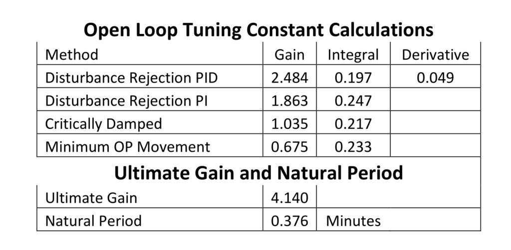
Don’t read too much into the precision of these tuning constants. It is very difficult if not impossible to get a good step test of the process when other controllers interact with the controller being tested. This produces a complex response that may not fit the first order plus deadtime paradigm we’ve assumed for controller tuning. Regardless, we must start somewhere but recognize that the initial tuning constants are at best an educated guess.
Notch gap setup for a classical PID controller; velocity form
We already know that the controller gain inside the gap should be zero; we are only worried about how the controller will respond when the PV hits the edge of the gap. Since the controller should nudge the process back inside the gap integral should be emphasized to push the controller output to a new value and gain should be deemphasized. This would suggest using a controller gain about equal to minimum OP movement and using the fastest recommended integral constant. We are looking for a controller response where the OP is adjusted only occasionally.
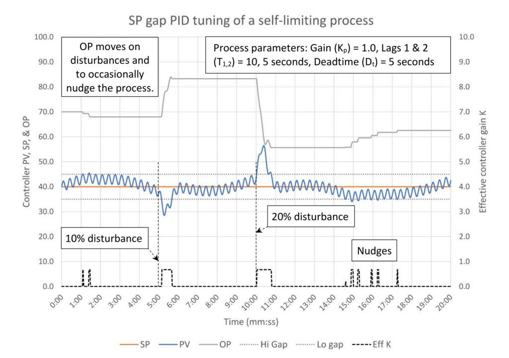
In Figure 10 the pressure controller is behaving as desired. It knocks down 10% and 20% disturbances at the 5 and 10 minute marks, otherwise it mostly doesn’t nudge the controller output unless the normal movement of the PV requires it. Even then the nudges are fairly small. The controller tuning is not very aggressive to minimize the chance of persistent interaction with the flow controllers.
Naturally, in the real world you would not expect to see this many disturbances this close together. Normally you would expect to see fewer nudges. You could consider widening the controller gap as long as the gap doesn’t violate any process constraints to reduce the number of nudges. Also, a process that is this active would warrant a closer look at the tuning of the combustion control system. There is certainly plenty of room for optimization depending on the process, so feel free to work with the tuning as necessary.
Floating setpoint gap setup for a parallel PID controller
Planning a floating gap controller setup is the same as a notch gap controller setup; you set the gap and set the tuning to deemphasize controller gain and speed up integral.
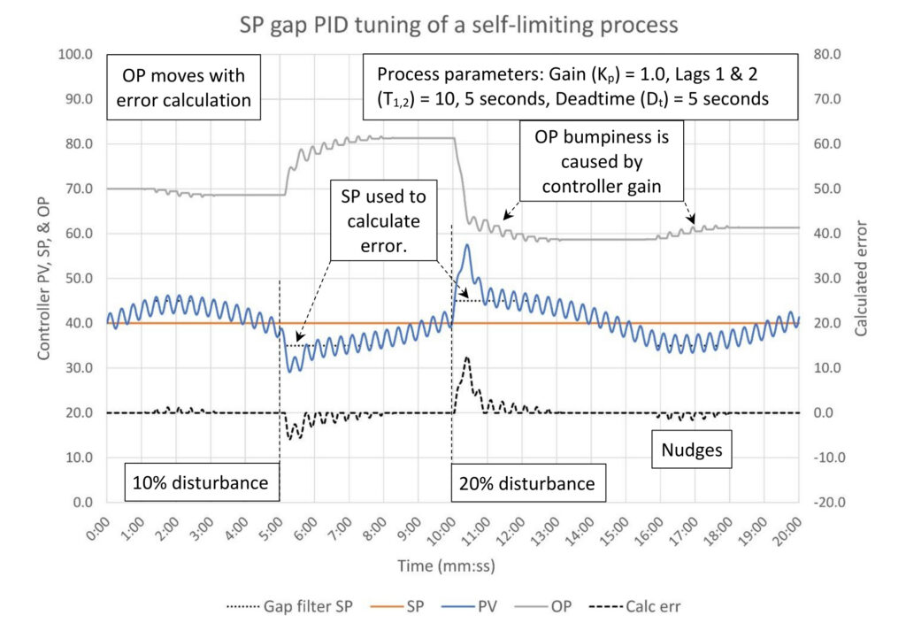
The floating SP gap controller in Figure 11 uses the same tuning as the notch gap controller in Figure 10 but has somewhat different results. The controller does correct the disturbances and nudges the process back within the gap when it drifts out, but the nudges are quite bumpy. We would prefer to stay away from this behavior if possible. Since controller gain is responsible for the OP movement mirroring the PV movement on the bumps, we should see if reducing the controller gain and speeding up the integral will remove the bumpiness.
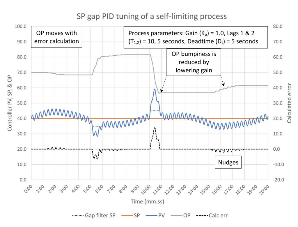
Reducing the controller gain and speeding up the integral as seen in Figure 12 did considerably reduce the bumpiness of the controller output movement. The logical endpoint of this is to eliminate controller gain altogether, which will require using the integral only version of the PID classical controller (assuming it’s an option on the system) or the parallel PID controller.
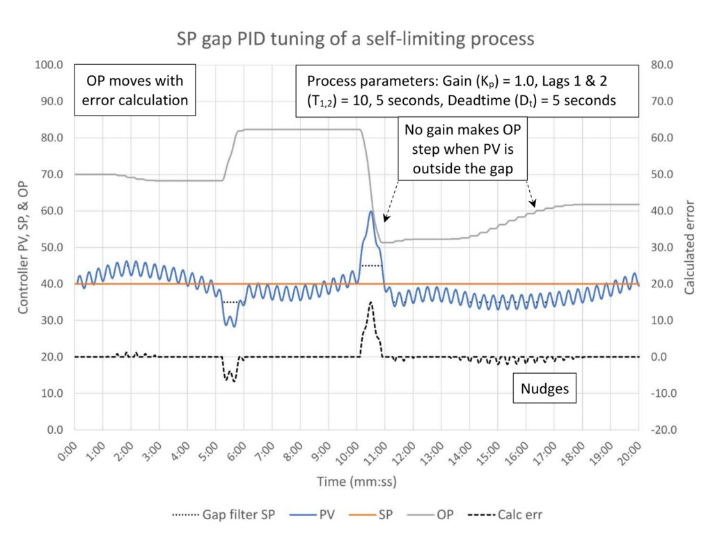
To eliminate controller gain Figure 13 uses a parallel PID controller tuned with controller gain set to 0 and integral set at 5.0 repeats/minute. Eliminating the controller gain yields the controller performance we are looking for; whenever the PV moves outside the gap, the OP moves enough to push it back inside the gap. Although for this process (that can result in a string of nudges), it still does a good job of correcting the two disturbances.
Just for background, the floating SP gap algorithm was developed for the parallel PID algorithm and is almost exclusively tuned integral only for these types of gap applications. Its application to the classical PID algorithm will have some less desirable behavior due to the requirement to have some controller gain.
Ed Bullerdiek is a retired control engineer with 37 years of process control experience in petroleum refining and oil production. Send comments and questions to [email protected]. Edited by Mark T. Hoske, editor-in-chief, Control Engineering, Arrowfly, [email protected].
Keywords
Proportional-integral-derivative, PID tutorial
Learning objectives
- Know that setpoint gap control can be used to shape controller response for better control of large disturbances, constraint control, and controllers that interact.
- Understand that setpoint gap control is only useful for lag/deadtime ratios greater than 1:1.
- Understand which setpoint gap control algorithm should be used based on the PID controller algorithm and the control problem to be solved.
- Know how to set up the setpoint gap controller understand the problems that may occur during tuning.
Consider this
Many situations come up where we want to shape PID controller response. We want faster response when a large disturbance comes through or when the process wanders close to a constraint but at the same time a more relaxed response to smaller disturbances or when the process is safely away from a limit. Or we may just need a way to break interaction between controllers while still keeping the process within reasonable limits. Setpoint gap action may allow us to do these things when set up properly.
You also might like
PID series from Ed Bullerdiek, retired control engineer
PID Spotlight, part 1: Three reasons to tune control loops: Safety, profit, energy efficiency
PID spotlight, part 2: Know these 13 terms, interactions
PID spotlight, part 3: How to select one of four process responses
PID spotlight, part 4: How to balance PID control for a self-limiting process
PID spotlight, part 5: What does good and bad controller tuning look like?
PID spotlight, part 6: Deadtime? How to boost controller performance anyway
PID spotlight, part 7: Open-loop tuning of a self-limiting process
PID spotlight, part 8: Closed-loop tuning for self-limiting processes
PID spotlight, part 9: Heuristic tuning for a self-limiting process (part A on heuristic tuning)
PID spotlight, part 10: Heuristic tuning in a self-limiting process
PID spotlight, part 11: How a PID controller works with an integrating process
PID spotlight, part 12: What does good and bad controller tuning look like?
PID spotlight, part 13: Deadtime: what’s the best that I can do?
PID spotlight, part 14: Open loop tuning of an integrating process
PID spotlight, part 15: Open loop tuning of near integrating processes
PID spotlight, part 16: Closed loop tuning of an integrating process
PID spotlight, part 17: Heuristic tuning of an integrating processes
PID spotlight, part 18: Identifying control valve performance problems
PID spotlight, part 19: PID controller tuning mechanics
PID spotlight, part 20: Tuning with bad valves
PID spotlight, part 21: Noise: Can I tune around it?
PID spotlight, part 22: Can I tune a noisy PID controller?
PID spotlight, part 23: Filtering noise for better PID control
PID spotlight: part 24: How do I tune PID controllers during a new unit startup?
PID spotlight, part 25: Navigating PID controller tuning
PID spotlight, part 26: How fast should I tune my PID controller?
PID spotlight, part 27: Navigating PID controller tuning
PID spotlight, part 28: How well will my PID controller work?
PID spotlight, part 29: How to shape PID controller response – part 1
PID spotlight, part 30: How to shape PID controller response – integrating processes
PID spotlight, part 31: What is PID gap control?
More on PID and advanced process control from Control Engineering