What is filtering? How does it work? How do we integrate it into the PID controller tuning process?

Insights about how to filter process noise for better PID control
- Filtering for noise can improve PID controller performance, but it can also require slower tuning. Finding the best tradeoff between filtering and controller tuning for best performance can be an iterative process.
- The type of filter you use can depend on the type of noise you have.
- There are handy guidelines for setting the filter time constant, however there are situations where the guidelines can be ignored.
Process noise can negatively impact PID controller performance, and it complicates tuning PID controllers, as we learned in PID spotlight parts 21 and 22. In short, we have to do something to hide (or ignore) the noise while keeping the actual process response.
The most common approach to hiding process noise is to apply a “low pass” filter. This is a fancy way of saying we are going to use a running or moving average of the last X measurements, which has the effect of filtering out fast (high frequency) noise while passing the slow (low frequency) process signal (hence the name low pass filter).
Unfortunately, a low pass filter does not provide a crisp cut between noise and process response. Of course, if you have a very slow process then you can apply a lot of filtering with little impact on controller performance. However, if you have a fast process then filtering will impact controller performance. In these latter cases you will need to make a tradeoff; how much filtering can you add to fix the performance problems noise can create without adding so much filtering that the filtering creates its own performance problems?
Filtering white noise

Figure 1 shows how a first order lag filter and a moving average filter attenuates normally distributed white noise. A relatively small amount of filtering can produce a significant reduction in noise. A first order filter achieves about a 70% reduction at 6 seconds. A moving average filter achieves 70% at 12 seconds. Adding more filtering in either case rapidly results in diminishing returns.
It appears that for true white noise a first order filter is our best option, and it should be limited to no more than about 10 seconds. (Let’s state for the record that you will rarely encounter true white noise; you may have to use more filtering. But the basic premise stands; a little bit of filtering helps a lot, adding more doesn’t help as much.)
Filtering cyclic noise
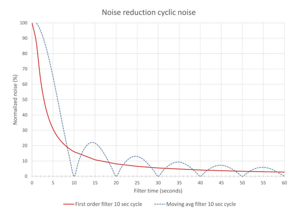
Cyclic noise, whether sine wave or other wave form, responds differently to first order and moving average filters. In Figure 2 the noise attenuation of a first order filter looks the same as white noise; there is a rapid drop toward 70% reduction at the 5 second mark followed by rapidly diminishing returns for additional filtering. The moving average filter eliminates the noise signal if the filter period is a multiple of the cycle period (the attenuation curve looks like a bouncing ball).
I have never used a moving average filter simply because refining doesn’t have processes where cyclic noise can be expected. Note also that most control equipment supports adding a first order filter (so does most instrumentation) whereas adding a moving average filter requires additional programming. Furthermore, the moving average calculation may lose important process variable information like instrument status.
That said, if you have a process with a cyclic noise component then it may be worth your while to consider using a moving average filter. If you choose to stick with a first order filter noise attenuation is proportional to the cycle time. The best tradeoff on filtering is to set the filter time equal to the cycle time. In this case 10 seconds is about the best. If you have a 30 second cycle set the first order filter time to 30 seconds.
How does filtering affect the process?
Adding a filter affects how the controller sees the process. The process doesn’t change, however adding a first order filter looks to the controller like the process has an additional lag. This, of course, affects controller tuning; making the process appear slower means we must slow down the controller tuning. If you are tuning for disturbance rejection the slower controller tuning will allow larger and longer lasting disturbances. Whether or not this will be a problem depends on how fast the process is.
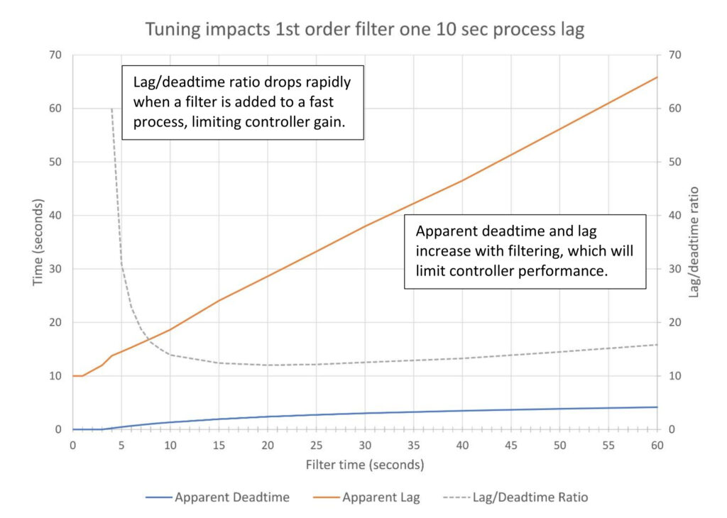
Figure 3 shows how a first order filter affects the apparent deadtime and lag of a very fast process; one with one 10 second lag and no deadtime. The process itself has an infinite lag/deadtime ratio, which means we could set the controller gain as high as the controller will permit and still have stable control. If we are looking for extremely tight control, a high controller gain may be necessary.
However, once we start adding a filter, the apparent lag rises rapidly from 10 to near 20 seconds when the filter reaches 10 seconds. A filter time beyond 10 seconds dominates the apparent “process” response. Worse yet, when the filter exceeds 3 seconds, we start to see the apparent deadtime increase. This causes the lag/deadtime ratio to rapidly decrease to about 14 when the filter time reaches 10 seconds. A lag/deadtime ratio of 14 tells us our controller gain should be no more than 7 times the baseline controller gain. Depending on the controller performance you need, this could be a problem.
The fix for this is to lower the filter time, however, this will increase noise. More noise means we have to live with the controller performance limitations and tuning issues we identified in the previous two articles.

Figure 4 presents a much different picture of how a filter will affect the apparent process. This is a process with three 30 second lags, which has an apparent deadtime of 22 seconds and an apparent lag of 74 seconds for a lag/deadtime ratio of 3.3. The maximum stable controller tuning for this process has a moderate ability to eliminate process disturbances; we can expect that adding filtering will negatively impact tuning.
Adding a filter rapidly raises the apparent deadtime, lowering the lag/deadtime ratio. The lag/deadtime ratio drops as low as 2.2 when the filter time reaches 25 seconds. Even if we use the quick start filter guide (PID spotlight part 21) and set the filter to one-tenth the apparent lag (7 seconds) the lag/deadtime ratio is 2.7, and the maximum gain we can use on the controller is 20% lower.
Our takeaway from this is if controller performance is a concern, then if noise filtering is required, we will have a balancing problem for fast and even some moderately slow processes. Rules of thumb may not provide sufficient guidance. However, if performance is not an issue or the process is very slow, then filtering within reason will not cause a problem.
About those filter guidelines
There are multiple opinions on how to set the first order lag filter constant (Tfilter). Suggested options are:
- Tfilter < T1 / 10 (One-tenth the process lag)
- Tfilter < Ti / 10 (One-tenth the integral tuning constant)
- Tfilter < Dt / 5 (One-fifth the process deadtime)
If you do an open loop test then setting the filter constant to no more than one-tenth the process lag is simple. If, however, you determine your tuning constants using closed or heuristic methods then setting the filter to no more than one-tenth the integral constant works. If you have a deadtime dominant process you may be better served setting the filter to no more than one-fifth the process deadtime.
Regardless, these should not be considered hard and fast rules. A very fast process such as our first example with no deadtime and a 10 second lag would allow you no more than a 1 second filter. Depending on the severity of the noise this may not be adequate. You may be forced to make a compromise. In simulation it appeared that a 6 second filter was required to bring a +/-10% white noise band to a reasonable level. The controller gain was reduced by 75%, and integral was sped up 17%, which still achieved good disturbance rejection.
Our second example with three 30 second lags was tuned for disturbance rejection with a controller gain of 1.67, integral of 1.125 minutes/repeat and derivative of 0.28 minutes. A 10% mixed noise band (5% white, 5% cyclic with a 10 second cycle) worked reasonably well with a 10 second moving average filter (matching the cycle), however the derivative constant had to be reduced to 0.10 after adding a 6 second derivative filter. This resulted in slightly more oscillatory control.
Derivative filter
Some control systems allow you to filter the derivative response. Because derivative multiplies noise adding a filter just to the derivative allows you to focus the noise reduction to just the derivative. Most systems implement the filter as a first order lag and set the filter time constant as a fraction of the derivative time. Guidance is to set this ratio between 0.1 and 0.2 (divide derivative time between 5 and 10).
I have not worked with derivative filtering outside of simulations. However, it appears to be a powerful tool to allow us to use derivative when noise is present. Also, based on the simulations, the guidance is more a suggestion than a hard and fast rule.
Tuning and filtering example 1
Because filtering for noise interacts with tuning, there isn’t a strictly linear process to get to a set of final tuning and filtering constants. There is likely to be some back and forth before you arrive at your best solution. In general, if you walk up to a noisy process your first step will be to set some kind of filtering. If the situation permits make a step test.
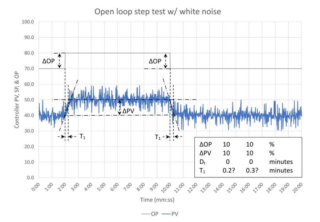
Figure 5 is a step test of our process with a single 10 second lag and no deadtime. We can see that the process gain is 1.0. After that it looks like there is no deadtime, and the process lag is 0.2 or 0.3? The lag looks like it is somewhere in the range of 12 to 18 seconds… maybe.
If we don’t need aggressive tuning, we could set the filter time at 4 to 5 seconds, retest and accept that the tuning will not provide the best possible disturbance rejection. If, however, we need better performance, we would start with our filter guidelines and set the filter at one-tenth our best guess at the process lag or 1.5 seconds.
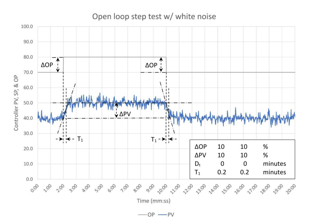
There is still a fair amount of noise in Figure 6, but it looks like we can settle on about 0.2 minutes for the process lag. The calculated tuning constants using the simplified IMC method are (see PID spotlight part 7):
K = 4
Ti = 0.15
Td = 0.04 (if used)
We will not use derivative, because it multiplies noise. We should also expect that the high controller gain will result in excessive controller output (OP) movement.

We can see in Figure 7 that while we have excellent disturbance suppression, the only way we know one happened is due to the controller output (OP) movement, but as we suspected the controller gain causes the OP to move excessively. It’s time to work on a suitable tradeoff. This could take multiple steps, and the final result will depend on your preferences. The next figure is final based on my preferences.
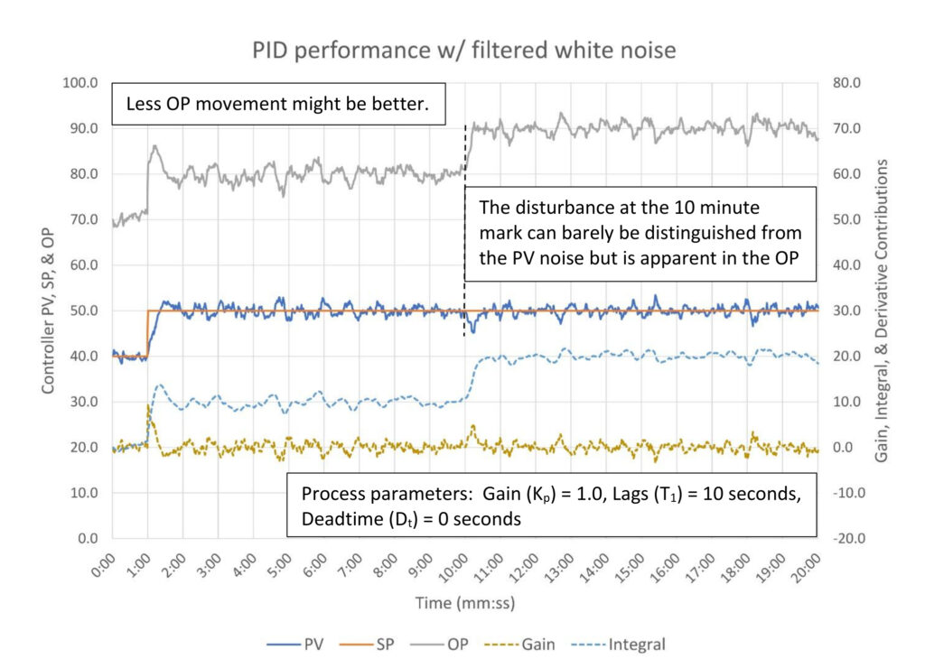
Figure 8 is my best compromise between performance and controller output movement. As expected, based on what we learned in PID spotlight part 21 controller gain was lowered by 75%, and integral was sped up slightly (17%). The noise filter was increased to 6 seconds to get a handle on the extreme process noise. The controller gain contribution plot shows how filtering and lowering the controller gain has largely tamped down the controller response to noise. The integral contribution plot shows that the integral is set so fast that it is chasing noise a bit, which is a tradeoff to get the controller to respond very quickly to the disturbance at the 10 minute mark.
The filter constant is 0.8 of the integral constant, far higher than the guideline that the filter constant should be no more than 0.1 of the integral constant. This is an extreme case and shouldn’t be something that you normally do. However, flows have fast dynamics and are often very noisy; you may find yourself bending the rules to get acceptable performance with many flow controllers.
Tuning and filtering example 2
Our second process is considerably slower than the first process. It also has multiple lags, which gives it significant apparent deadtime and also makes it a candidate for using derivative. This process also has mixed noise which includes a cyclic component as well as white noise. As with example one we will begin with a step test.
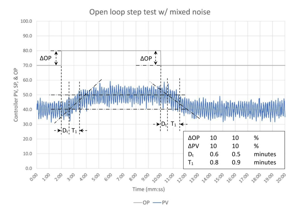
The first thing that stands out in Figure 9 is the cyclic nature of the noise. We can easily count 6 peaks/minute, which suggests that the cyclic noise has a 10 second period. At this point we should take a deep look at the process to verify that there is a legitimate reason for the cycle. If we cannot find one, we should look for an equipment fault and, if possible, get it repaired. We should fix problems, not cover them up. Otherwise, we run the risk that whatever is causing the cyclic noise will change cycle time or disappear altogether, which will make our filtering less effective.
We can also see from the steps that the deadtime looks like it might be half a minute and the apparent lag a little less than a minute. But before we start to make any tuning calculations, let’s add a 10 second moving average filter to eliminate the cyclic noise and help suppress the white noise.
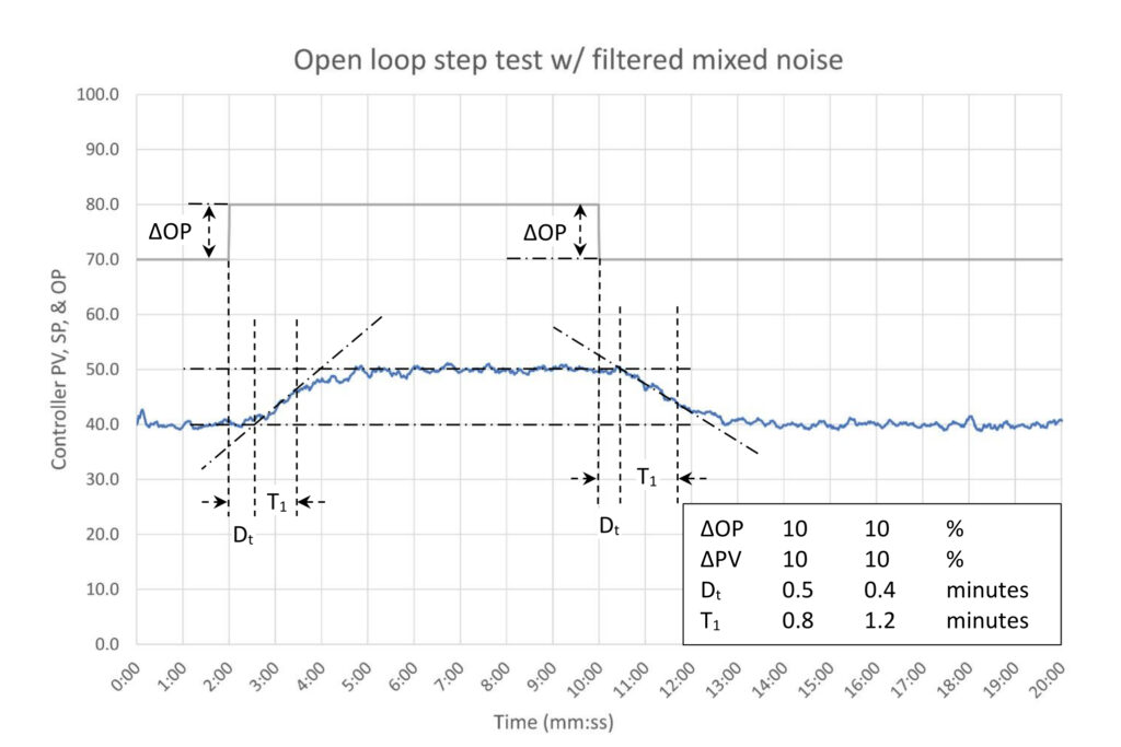
From the looks of Figure 10 the 10 second moving average filter did an excellent job of eliminating the cyclic noise and tamping down the white noise. It’s time to calculate tuning constants based on an estimated 0.5 minutes deadtime and a 1 minute process lag (and baseline gain of 1.0). Using the simplified IMC tuning calculations (PID spotlight part 7) we get:
K = 1.67
Ti = 1.125
Td = 0.28 (if used)
We will start without derivative.
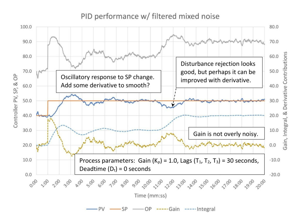
In Figure 11 there is some oscillation after the setpoint change. Since we are pursuing aggressive disturbance rejection tuning, we would like to add some derivative to tamp down the oscillation and provide a quicker response to the disturbance at the 10 minute mark. Let’s set the derivative to one-fourth the integral per normal tuning guidelines, or 0.28.
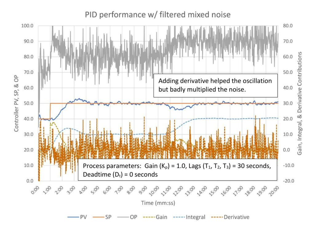
In Figure 12 adding derivative has tamped down the process variable (PV) oscillations after a setpoint (SP) change like we wanted. It is difficult to tell from the PV trend if the response to the disturbance has been improved. However, the noise multiplier effect of derivative is driving the controller output (OP) all over the place. We’re going to have to do something about this. Let’s begin by setting the derivative filter per the guidelines, or 0.2 times 0.28 minutes, which is 3 seconds.
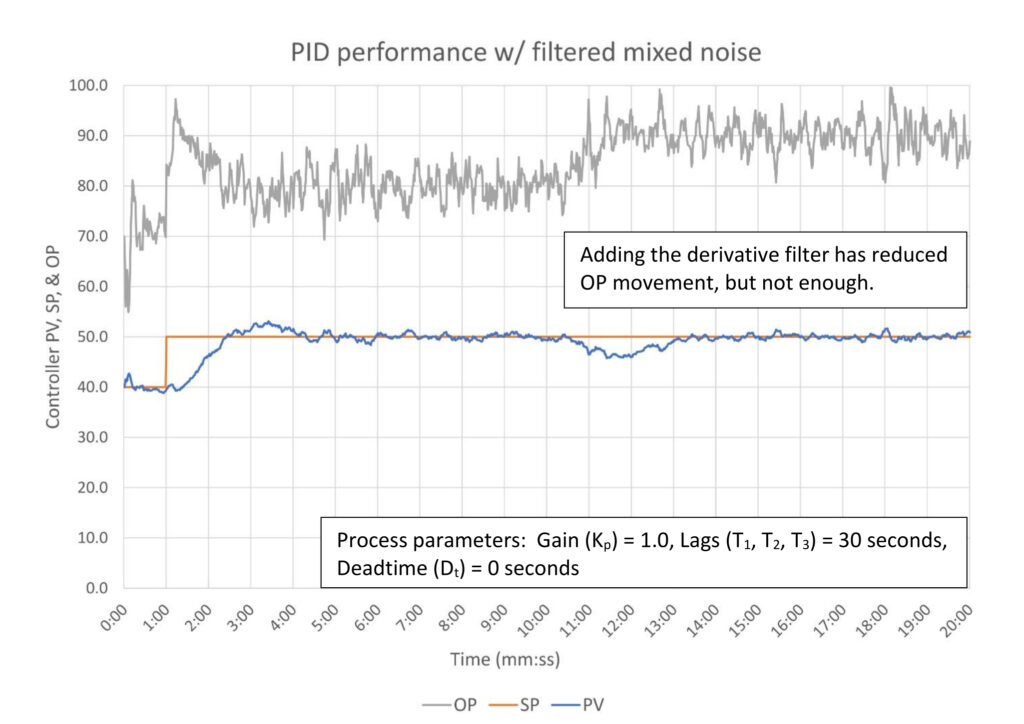
Adding the derivative filter did reduce controller output movement in Figure 13, however, the relatively modest amount of noise is still causing significant valve movement. Following the guidelines in this admittedly extreme case isn’t working. We should be able to reduce the derivative and possibly raise the derivative filter and retain the benefits of having some derivative without the problems caused by the process noise. This will be an iterative process, and the next chart is my best guess at an optimal solution.

Figure 14 shows my best guess at the minimum derivative constant and derivative filter that will give us the performance that we would like. I chose a 6 second filter to get an estimated 70% reduction in white noise and set the derivative to 6 seconds (0.1 minutes). Most systems will not let you set the derivative filter ratio greater than 1, which is a reasonable constraint. A derivative of 0.2 and derivative filter of 12 seconds also works.
Summary of filtering process noise for PID tuning
Filtering process noise may be necessary to permit proper tuning and operation of a PID controller and prevent unwanted control valve movement. However, filtering does not come without tradeoffs. Adding a first order or moving average filter adds apparent process deadtime and lag to the system, which can limit how aggressively a controller is tuned. This will likely not be an issue for very slow processes, but could be significant for fast processes or processes with low lag/deadtime ratios.
A process noise filter rapidly reduces noise at small values, but the effect of increasing the filter time diminishes rapidly.
There are guidelines for setting filter constants, however, these guidelines are not hard and may be exceeded when necessary.
Using a derivative filter can preserve the advantages of derivative action while mitigating the effect of derivative multiplication of noise on control valve movement.
Ed Bullerdiek is a retired control engineer with 37 years of process control experience in petroleum refining and oil production. Edited by Mark T. Hoske, editor-in-chief, Control Engineering, WTWH Media, [email protected].
Keywords
Proportional-integral-derivative, PID tutorial
Learning objectives
- Know that a little filtering rapidly reduces noise; adding more has diminishing returns. Also know when to use a first order or moving average filter.
- Understand that adding a filter may adversely impact PID controller performance. You may have to make tradeoffs between filtering and tuning to optimize performance.
- Know the filter guidelines; understand when they may be ignored. Understand filtering derivative action of a controller.
Consider this
Filtering may be necessary to improve PID controller performance, but may also negatively affect PID controller performance. What tradeoffs might you have to make to get good control?
PID series from Ed Bullerdiek, retired control engineer
Part 1: Three reasons to tune control loops: Safety, profit, energy efficiency
PID spotlight, part 2: Know these 13 terms, interactions
PID spotlight, part 3: How to select one of four process responses
PID spotlight, part 4: How to balance PID control for a self-limiting process
PID spotlight, part 5: What does good and bad controller tuning look like?
PID spotlight, part 6: Deadtime? How to boost controller performance anyway
PID spotlight, part 7: Open-loop tuning of a self-limiting process
PID spotlight, part 8: Closed-loop tuning for self-limiting processes
PID spotlight, part 9: Heuristic tuning for a self-limiting process (part A on heuristic tuning)
PID spotlight, part 10: Heuristic tuning in a self-limiting process
PID spotlight, part 11: How a PID controller works with an integrating process
PID spotlight, part 12: What does good and bad controller tuning look like?
PID spotlight, part 13: Deadtime: what’s the best that I can do?
PID spotlight, part 14: Open loop tuning of an integrating process
PID spotlight, part 15: Open loop tuning of near integrating processes
PID spotlight, part 16: Closed loop tuning of an integrating process
PID spotlight, part 17: Heuristic tuning of an integrating process
PID spotlight, part 18: Identifying control valve performance problems
PID spotlight, part 19: PID controller tuning mechanics
PID spotlight, part 20: How to tune with sticking control valves
PID spotlight, part 21: Noise: Can I tune around it?
PID spotlight, part 22: Can I tune a noisy PID controller?
More on PID and advanced process control from Control Engineering