What measures of PID controller performance should we care about? How do our tuning choices affect performance? Does the process lag/deadtime ratio limit how well a PID controller can perform, and can we estimate performance?

Insights about estimating PID controller performance
- There are four industrially relevant measures of PID controller performance: disturbance rejection effectiveness, disturbance arrest time, disturbance recovery time and time to new setpoint.
- Lag/deadtime ratio has a large impact on best possible controller performance. Lag dominant processes can be very effectively controlled by a PID controller. Deadtime dominant processes cannot be effectively controlled. The zone between lag and deadtime dominant processes has a very quick transition between effective and ineffective control.
- Controller gain is the primary knob for controlling disturbance rejection effectiveness and arrest time. Integral controls disturbance recovery time. An appropriate combination of controller gain and integral determines the time it takes for a controller to settle on a new setpoint.
When we decide to tune a proportional-integral-derivative (PID) controller, we might like to be able to estimate performance. Admittedly when I sit down to tune I never say, “I need 50% disturbance rejection.” Usually we will tune first, and if the controller works well enough, we log the constants and move on to the next task. We don’t want to work any harder than we have to.
This will only become important when we come to the hard cases, which, hopefully, are rare. Either we are having a hard time getting the performance that we need, or we have a situation where exceeding a specific limit will have undesirable results. In these cases it will be useful to be able to estimate what performance we can get out of the controller, and what moves we have to make to increase performance. We also may find that our PID controller alone cannot meet our needs, and we must find ways to help our controller.
How well can a controller perform based on lag/deadtime ratio and tuning style? There are several useful measures of performance we can estimate from the lag/deadtime ratio of a self-limiting process. These are:
- Disturbance rejection effectiveness
- Disturbance arrest time
- Disturbance recovery time
- Time to a new setpoint
All four of these are affected by how you tune the PID controller.
Disturbance rejection effectiveness
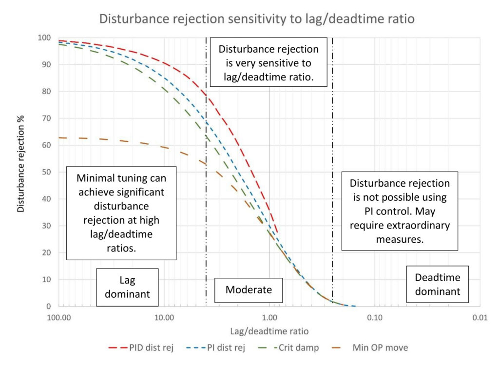
Figure 1 plots disturbance rejection effectiveness for PID and PI disturbance rejection, critically damped and minimum controller output movement tuning. Disturbance rejection effectiveness is primarily controlled by controller gain followed by integral at lower lag/deadtime ratios. Adding derivative can help both by speeding response to a disturbance and allowing higher controller gain and faster integral without oscillation. If disturbance rejection is your primary goal increase controller gain.
At high lag/deadtime ratios (>10:1) even minimum controller output movement tuning will net a 60% reduction in disturbance size. In these cases, you have a lot of leeway to reduce controller gain to reduce disturbances to other parts of the process while preserving adequate performance.
At low lag/deadtime ratios (<1:4) a PID controller cannot prevent a disturbance from being fully expressed and persistent. (Fully expressed means that if a disturbance would cause a 10% change in the PV when the controller is turned off, it will also result in a 10% change when the controller is in service.) Fundamentally the deadtime is so long that controller cannot catch the disturbance; it is doomed to perpetually play catchup.
Between the lag dominant and deadtime dominant lag/deadtime ratios, there is a rapid transition from easily being able to suppress disturbances to a complete inability to suppress disturbances. Furthermore below a lag/deadtime ratio of about 1:1 there is little difference between tuning for disturbance rejection and minimum controller output movement. There’s little you can do with controller gain at this point because the ceiling on stable controller gain is so low.
It’s important in this range, especially since many of the processes we run into will have lag/deadtime ratios in this range, to avoid adding unnecessary deadtime. We’ve mentioned using filters to reduce process noise, but this also includes deadtime that can be caused by instrument placement, control valve issues, and seemingly innocuous items like controller execution interval, control system internal scheduling and communications latency. Everything adds up and can wreck what should have been acceptable performance.
Disturbance arrest time
The vertical scales in figures 2 through 6 must be multiplied by the process deadtime (Dt) to get the final time, whether it is disturbance arrest time (Ta), disturbance recovery time (Tr) or time to setpoint (Tsp).
T? = T?X * Dt
No correlations were developed as the times are sensitive to tuning and the simulation used to develop the data has a 1 second execution interval. The data resolution is no better than 1 second, and you will see that the closeup trends are rather choppy as a result. Regardless, the charts are good enough for a general discussion of how tuning affects controller response.
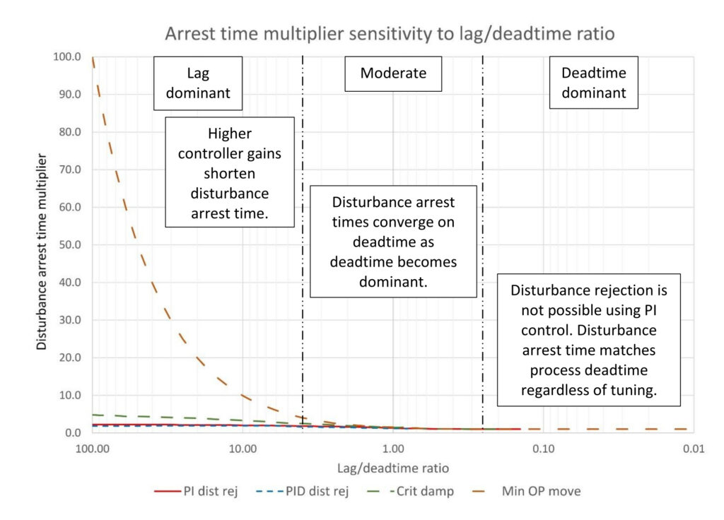
In Figure 2 we can see that the disturbance arrest time for minimum controller output (OP) movement tuning matches the process lag time at high lag/deadtime ratios. The steadily higher controller gains employed by the other three methods considerably shorten arrest time.
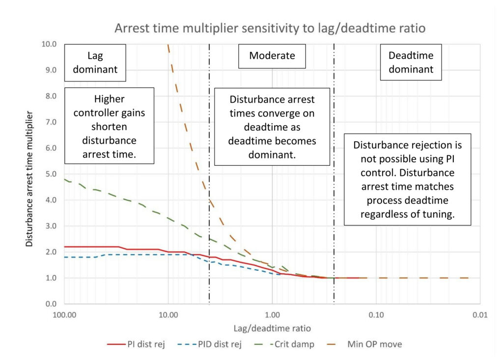
The closeup view of Figure 3 clears up some of the details. At higher lag/deadtime ratios deadtime and lag both contribute to arrest time. Deadtime, of course, completely stops the process response to controller action whereas lag merely delays it. Lag can be overcome by increasing controller gain, with the potential penalty of eventual overshoot. It appears that even critically damped tuning can manage arrest time reasonably well and by its very nature will not produce much process variable overshoot over setpoint, nor will the controller output overshoot its final value when a disturbance occurs.
Note that the arrest time trended here was for critically damped tuning that produced 5% overshoot. Tuning that aims for less overshoot will extend arrest time.
As the process trends toward deadtime dominant disturbance arrest time settles on the deadtime. This is something of a misnomer as for deadtime dominant processes the disturbance is fully expressed and persistent before the process can respond to anything the controller can do. It’s not so much “disturbance arrest” time as much as it is “now we can start to fix this mess” time since the mess has already been made.
Disturbance recovery time
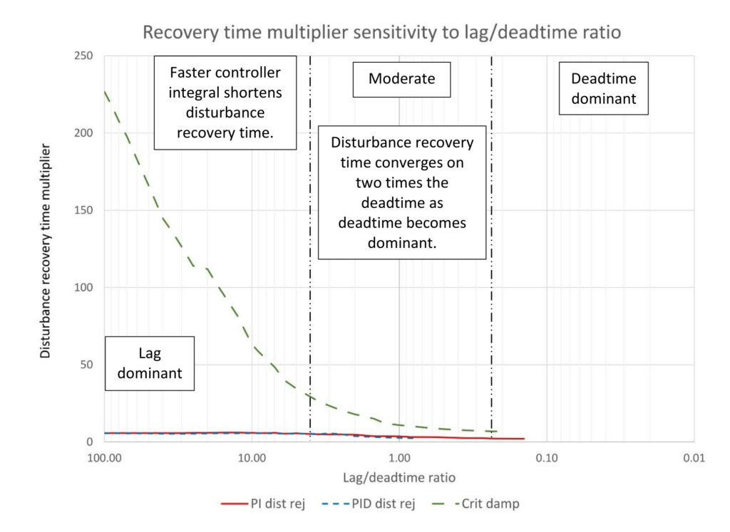
Disturbance recovery time is different than disturbance arrest time because it is more affected by integral than controller gain. Figure 4 shows that critically damped tuning, because its integral is considerably slower than disturbance rejection tuning, has a considerably longer disturbance recovery time despite having a relatively similar disturbance arrest time. This can be modified considerably by changing the integral constant, but as with disturbance arrest time speeding up integral will increase overshoot.
Minimum controller output movement tuning is not included. It can be estimated at four times the lag time if the need exists.
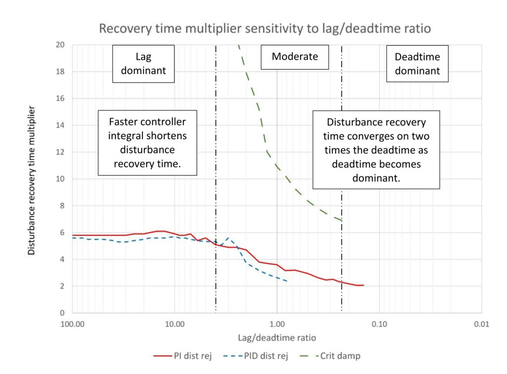
Figure 5 gives us a closer look at disturbance rejection recovery time. Ideally disturbance recovery time should be twice disturbance arrest time if the process variable (PV) response was truly symmetrical. My personal preference to avoid secondary oscillations left the PI disturbance response time at closer six times deadtime as opposed to the four you would expect based on the disturbance arrest time multiplier of two. This is a preference you may choose to emulate or not.
The PID disturbance response story is a little different. Derivative penalizes PV movement, so it has the tendency to slow the recovery time regardless of integral. This is a small tradeoff for the improved disturbance rejection efficiency you can get using derivative.
Time to setpoint
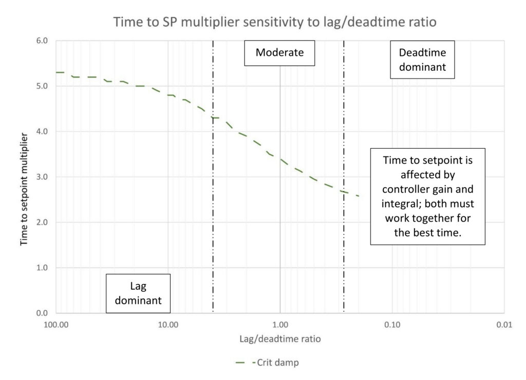
Figure 6 shows that the time for the process variable to reach setpoint after a setpoint change is about the same as the disturbance arrest time for a properly tuned critically damped controller. Controller gain and integral must be properly tuned to minimize time to setpoint without overshoot. Too much controller gain or if the integral is set too fast will result in overshoot. Controller gain set too small or integral set too slow needlessly extends time to setpoint. Mismatching can result in both overshoot and an extended time to settle on setpoint.
How well do the calculations work?
The controller tuning calculations and performance estimation data was developed using an ideal first order plus deadtime (FO+Dt) model with the exception of any calculations that required derivative. Presumably they will work well with a more real-world process model, but we won’t know until we try. Following are five tests, one each of the PID and PI disturbance rejection, critically damped, minimum controller output movement and simplified internal model control (IMC) PID calculations. These five tests were done on a process with a gain of 0.77 ΔPV/ΔOP (%/%), a deadtime of 18 seconds, and three lags of 80, 24 and 15 seconds. An open loop step test yields an effective deadtime of 40 seconds and process lag of 100 seconds for a lag/deadtime ratio of 2.5:1 and baseline controller gain (Kbase) of 1.3. A lag/deadtime ratio of 2.5:1 was chosen because it is in the range where sensitivity to lag/deadtime ratio is very high, which will make any inaccuracies stand out.
The minimum controller output (OP) calculations are also tested against a process with a gain of 0.77 ΔPV/ΔOP (%/%), a deadtime of 100 seconds and a lag of 40 seconds. This results in a lag/deadtime ratio of 1:2.5. This ratio is used to prove that the minimum OP movement calculations work accurately for a deadtime dominant process.
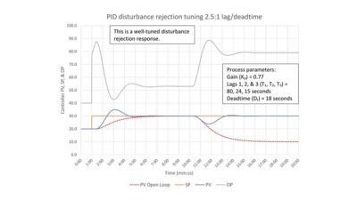
PID disturbance rejection:
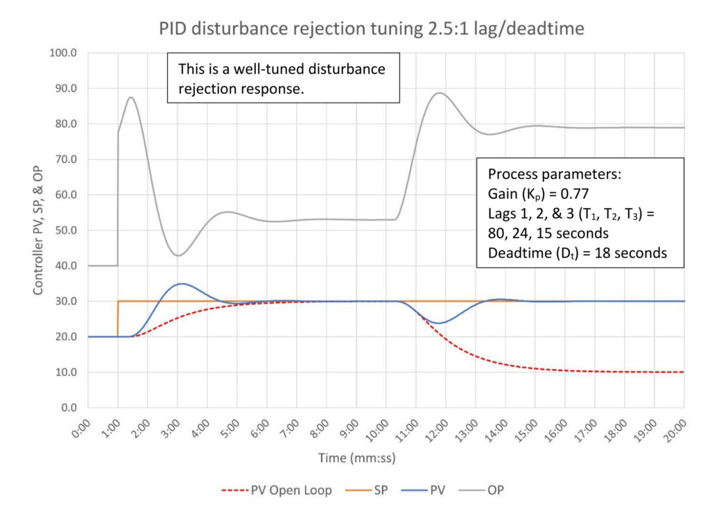
Figure 7: PID disturbance rejection tuning (2.5:1 lag/deadtime). Tuning constants are K = 3.7, Ti = 1.3 minutes/repeat, Td = 0.326 minutes. Courtesy: Ed Bullerdiek, retired control engineer
Figure 7 was tuned using the PID calculations in PID spotlight part 27 table 1. The response looks very good. Table 1 compares actual against estimated performance.
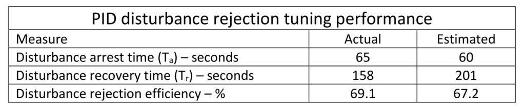
Disturbance arrest time was slightly worse than estimated. Disturbance rejection efficiency was slightly better and recovery time quite a bit better. Don’t put much weight on recovery time as this can be very sensitive to small changes in integral tuning. Overall our process with three lags and a small deadtime didn’t throw our tuning or estimation off.
PI disturbance rejection:
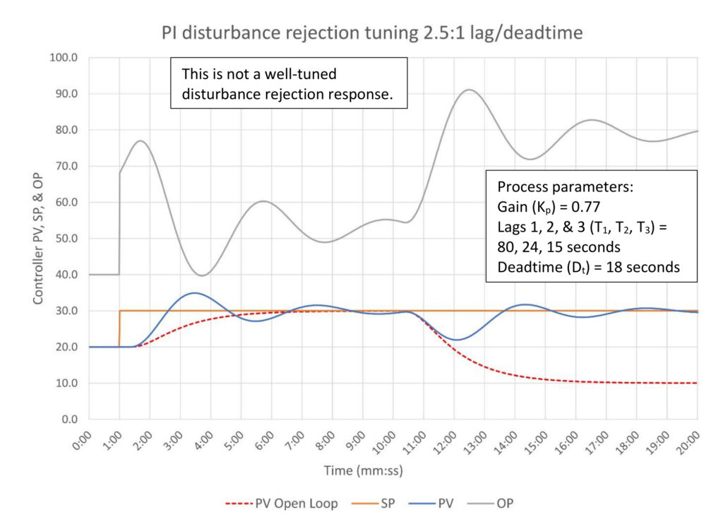
Figure 8: PI disturbance rejection tuning (2.5:1 lag/deadtime). Tuning constants are K = 2.78, Ti = 1.63 minutes/repeat, Td = 0 minutes. Courtesy: Ed Bullerdiek, retired control engineer
Figure 8 was tuned using the PI calculations in PID spotlight part 27 table 1 and, sadly, the PI disturbance rejection tuning didn’t fare very well. It looks very much like Ziegler-Nichols quarter amplitude damping tuning, which is far more aggressive than I prefer. A quick check of Z-N PI tuning for this process shows that the controller gain is the same, but the integral is slower at 1.98 minutes/repeat versus the 1.63 used here. Heuristics also tell us that the integral is too fast. Slowing the integral down to 2.25 minutes/repeat still had some oscillations, suggesting that controller gain might also be too large.
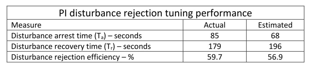
Interestingly, the disturbance arrest time is considerably worse, but the rejection efficiency is better than predicted (Table 2). Recovery time is slightly worse, but don’t put a lot of weight on that.
Adding a little bit of derivative (0.32 minutes) straightened the trend out. Note that this is only one-fifth the integral constant, not the one-fourth normally recommended. As expected, rejection efficiency got better (64.7%), arrest time got better (75 seconds) and recovery time got worse (198 seconds) due to the process variable movement penalty that derivative applies. Of course adding a little derivative is the easy button for knocking down oscillations assuming, of course, that your process isn’t noisy and has secondary lags.
To verify I hadn’t gone off the rails I double checked all the development work and found no issues. Then I converted the process to a true first order plus deadtime form (T1 = 100 seconds, Dt = 40 seconds), and the controller response settled into the pattern I was expecting. So clearly there is something about the three lags and shorter true deadtime that is fooling these calculations. This reinforces the idea that any calculation method may not yield ideal results and that they must be checked and adjusted as necessary.
Critically damped:
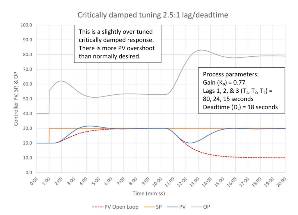
Figure 9: Critically damped tuning (2.5:1 lag/deadtime). Tuning constants are K = 1.542, Ti = 1.557 minutes/repeat, Td = 0 minutes. Courtesy: Ed Bullerdiek, retired control engineer
The controller in Figure 9 was tuned using the critically damped calculations in PID spotlight part 27 table 2. The controller response has just slightly more overshoot than we might desire, but this is admittedly a bit of a nitpick. In reality, depending on the process noise, you may not even notice the overshoot. Heuristics would suggest slowing down the integral just a little bit if this is an issue.
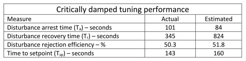
Table 3 compares critically damped tuning performance against expected. As with PID and PI, disturbance rejection tuning arrest time came in longer than estimated, suggesting that multiple lags may affect arrest time. Recovery time and time to setpoint are faster than expected, but this would be consistent with a slightly over tuned controller.
Minimum controller output movement:
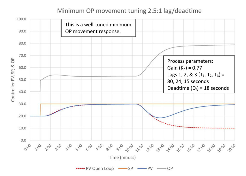
Figure 10: Minimum controller output (OP) movement tuning (2.5:1 lag/deadtime). Tuning constants are K = 0.918, Ti = 1.673 minutes/repeat, Td = 0 minutes. Courtesy: Ed Bullerdiek, retired control engineer
Figure 10 was tuned using the minimum controller output (OP) movement calculations in PID spotlight part 27 table 3. The response looks mostly like we would expect. Ideally the controller output would stop moving when the process variable started moving, but this depends on the PV having a crisp start. Multiple lags muddy up the PV start which results in the controller output having a muddy change in direction.
Out in the real world using minimum OP movement tuning on this process would be very unlikely. You would use it perhaps if this were a slow optimization situation, but this is somewhat aggressive for true slow optimization. You might instead use these calculations to put a ceiling on the highest controller gain and fastest integral you would use for slow optimization.

If we are doing slow optimization tuning, we are usually not worried about controller performance. The goal is to get there sometime, but not necessarily today. Regardless, in case you are interested, Table 4 shows us that arrest time is slower than estimated, and disturbance rejection efficiency isn’t as good as expected.
Simplified IMC PID:
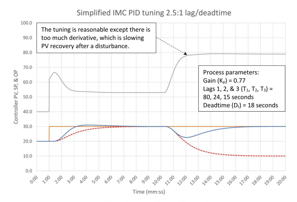
Figure 11: Simplified IMC PID tuning (2.5:1 lag/deadtime). Tuning constants are K = 2.198, Ti = 1.75 minutes/repeat, Td = 0.438 minutes. Courtesy: Ed Bullerdiek, retired control engineer
I’ve included Figure 11 to compare the simplified IMC PID tuning calculation introduced in PID spotlight part 7 with these latest calculations. The simplified IMC calculation is intended to provide serviceable tuning across the full range of lag/deadtime ratios as a default if you do not know exactly what you need. For this particular process, the PI calculations are slightly oscillatory so I chose to add derivative per the calculations to smooth the response. As it turns out, that is just a little too much derivative; the controller output is stopping short of its final value before drifting in. A slight reduction in derivative will clear up this problem.
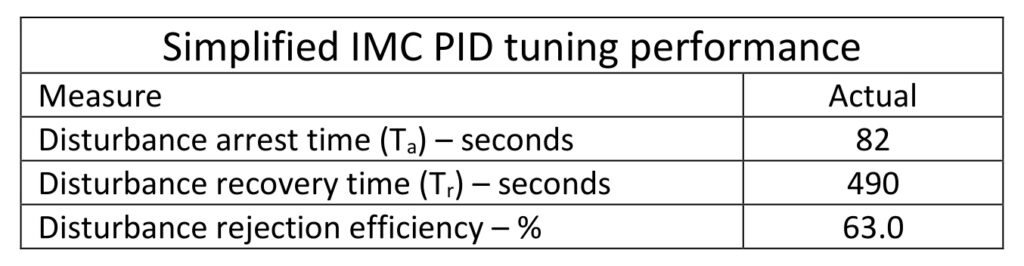
The actual performance is in Table 5. There is no estimated performance data for this tuning, but it is comparable to critically damped tuning.
Minimum controller output movement on a deadtime dominant process:
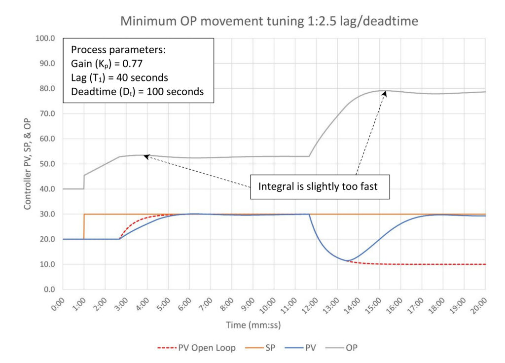
Figure 12: Minimum controller output (OP) movement tuning (1:2.5 lag/deadtime). Tuning constants are K = 0.536, Ti = 1.208 minutes/repeat, Td = 0 minutes. Courtesy: Ed Bullerdiek, retired control engineer
Figure 12 is included to illustrate how well the minimum OP movement tuning calculations work for a lag dominant process, since these are what this set of tuning equations are intended for. Integral is a little fast, resulting in slight output overshoot after the setpoint change and disturbance. This is easily cleaned up using heuristic methods. Regardless, getting this close from a step test is not a bad thing.
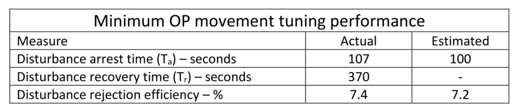
The controller performance is close to estimated (Table 6). As expected for a deadtime dominant process disturbance rejection efficiency is abysmal. At this point your only choices for better disturbance rejection are don’t let the disturbances in to begin with or provide some feedforward to get the controller moving before the disturbance occurs. If neither of these are possible, there are some tricks to improve recovery time, but even these have limitations.
Should we monitor controller performance?
Yes, some sort of monitoring should be done. How much and what type depends on the situation. If you are responsible for a handful of PID controllers you should look at the trends every once in a while. How often depends on how much the process might drift.
If you have a middling number of controllers (<100) and a data historian then at a minimum you should track time in proper mode (auto or cascade). You may also want to track operator interventions, how often an operator turns a controller off, makes a move, and then turns it back on. Operator interventions are a sign that the operator is “helping” the controller. If the controller needs frequent help, then you have an improvement opportunity in front of you. The controller may be too slow or perhaps there is a feedforward calculation that can be applied to save the operator some work. And, of course, paging through the trends and talking to the operators about how the process is running is never wasted time.
If you are in a large facility you might want to consider a controller performance monitoring package. My experience with these is mixed. They can dump a large amount of information in your lap every day. If you are particularly well versed in impulse plots and Bode diagrams, they can be particularly revealing. The most useful measures to me were the oscillation index and the settling time estimate. We don’t want anything to oscillate, nor do we want a controller to take an excessive amount of time to come back to setpoint after an upset or setpoint change.
Unfortunately, in our time-challenged world these can be time consuming. It takes time to customize the detection algorithm for each controller to make correct diagnoses. The packages come with a default setting for each process. For flows the default will likely be reasonable for most controllers as all flows should have similar dynamics, however, for every other process the defaults may not work well. Furthermore, refinery control system configurations are very dynamic. The configuration of the performance monitoring system must be updated to keep pace, or the system slowly becomes less useful. Unless there is a management commitment, and the personnel/money to back it up, it can become a lost investment. (For those of you rolling your eyes I, too, am very familiar with management indifference. In the right situation these could be very useful, but it must be the right situation.)
All that said, tuning doesn’t spontaneously break. The amount of monitoring you do should be keyed to how stable the process is. Refining involves high pressures and temperatures and dirty processes. This results in a lot of wear and tear as well as plugging of equipment; an environment where the process response drifts with time. If your process is stable the better approach might be to have a one-time analysis done to clean up the tuning followed by occasional checks of high-value controllers.
Ed Bullerdiek is a retired control engineer with 37 years of process control experience in petroleum refining and oil production. Send comments and questions to [email protected]. Edited by Mark T. Hoske, editor-in-chief, Control Engineering, WTWH Media, [email protected].
Keywords
Proportional-integral-derivative, PID tutorial
Learning objectives
- Know the four measures of PID controller performance.
- Understand how PID controller tuning affects each performance measure.
- Understand the relationship between lag/deadtime ratio and best possible PID controller performance.
Consider this
Knowing the relationship between the process lag/deadtime ratio, controller tuning and performance can help you get the best performance from your PID controllers.
You also might like
PID series from Ed Bullerdiek, retired control engineer
PID Spotlight, part 1: Three reasons to tune control loops: Safety, profit, energy efficiency
PID spotlight, part 2: Know these 13 terms, interactions
PID spotlight, part 3: How to select one of four process responses
PID spotlight, part 4: How to balance PID control for a self-limiting process
PID spotlight, part 5: What does good and bad controller tuning look like?
PID spotlight, part 6: Deadtime? How to boost controller performance anyway
PID spotlight, part 7: Open-loop tuning of a self-limiting process
PID spotlight, part 8: Closed-loop tuning for self-limiting processes
PID spotlight, part 9: Heuristic tuning for a self-limiting process (part A on heuristic tuning)
PID spotlight, part 10: Heuristic tuning in a self-limiting process
PID spotlight, part 11: How a PID controller works with an integrating process
PID spotlight, part 12: What does good and bad controller tuning look like?
PID spotlight, part 13: Deadtime: what’s the best that I can do?
PID spotlight, part 14: Open loop tuning of an integrating process
PID spotlight, part 15: Open loop tuning of near integrating processes
PID spotlight, part 16: Closed loop tuning of an integrating process
PID spotlight, part 17: Heuristic tuning of an integrating processes
PID spotlight, part 18: Identifying control valve performance problems
PID spotlight, part 19: PID controller tuning mechanics
PID spotlight, part 20: Tuning with bad valves
PID spotlight, part 21: Noise: Can I tune around it?
PID spotlight, part 22: Can I tune a noisy PID controller?
PID spotlight, part 23: Filtering noise for better PID control
PID spotlight: part 24: How do I tune PID controllers during a new unit startup?
PID spotlight, part 25: Navigating PID controller tuning
PID spotlight, part 26: How fast should I tune my PID controller?
PID spotlight, part 27: Navigating PID controller tuning
More on PID and advanced process control from Control Engineering