Do you need to stamp out disturbances as fast as possible? Or does rapid controller output movement cause problems with the rest of the process? Why should I tune a controller fast or slow?
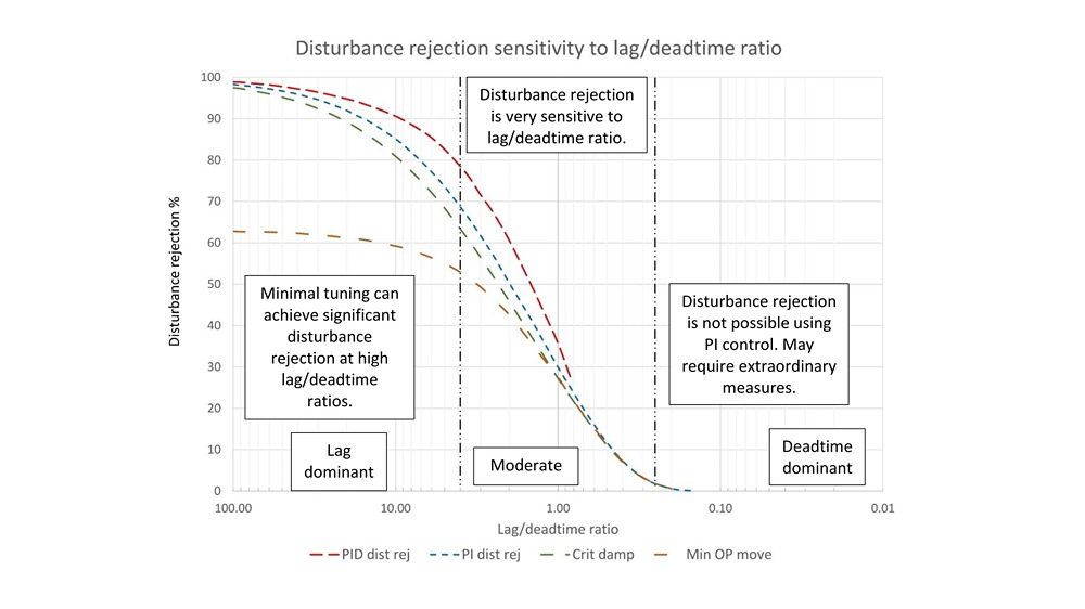
Insights about tuning for purpose.
- Optimal PID controller tuning starts with understanding how the controller fits in the entire process. Tuning of a PID controller exists on a continuum from very aggressive disturbance rejection tuning to very slow optimization tuning.
- Picking one of five tuning windows depends on how you weight disturbance rejection versus minimizing controller output movement to avoid disturbing other parts of the process.
- Published tuning methods have implicit tuning goals that may not meet the requirements for the controller you are tuning or may not work well at the lag/deadtime ratio of your process. Nor is there guidance on which method to pick to meet a specific goal.
When you sit down to tune a proportional-integral-derivative (PID) controller, the first question you should ask is: “What is this PID controller supposed to do? What, exactly, is its purpose?” To address this point we have focused on the mechanics of PID controller tuning because mastering these tools is necessary to the control tuner’s art, but we have only touched on the idea of tuning for purpose. Tuning for purpose will be covered in three articles:
- What is tuning for purpose? (this article)
- How do we find the controller tuning windows?
- How do we measure and predict controller performance?
Chemical processes are complex and with few exceptions every PID controller affects multiple other controllers. Because of this we need to weigh different aspects of controller performance, which include:
- How well does the controller correct disturbances to the process variable (PV)?
- How well does the process variable follow setpoint (SP) changes?
- Do changes to the controller output (OP) adversely affect other parts of the process?
- Is this controller supposed to perform slow optimization?
How you weight your answers to these four questions will direct you toward one of five controller tuning performance windows.
- Disturbance rejection, both PI and PID tuning (2 windows)
- Critically damped (aka setpoint following tuning)
- Minimizing controller output movement
- Slowly optimizing the process
One thing to keep in mind is if you give equal weight to (for example) critically damped (setpoint following) and minimizing controller output movement then it is perfectly acceptable to aim for controller performance between these windows. These are not straightjackets, merely a common definition of terms to be used to guide our thinking.
What is disturbance rejection tuning?
Disturbance rejection tuning is exactly as described; we tune the PID controller with the maximum controller gain and fastest integral possible to eliminate a process variable (PV) disturbance as fast as we can. If we really need to squeeze the last ounce of performance out of the controller, we will add derivative, which will allow us to increase controller gain and speed up integral even further. Tuning should minimize secondary oscillations to avoid unnecessary disturbances to the rest of the process.
Proportional-integral (PI) disturbance rejection tuning:
Figure 1 is an example of proportional-integral (PI) disturbance rejection tuning.
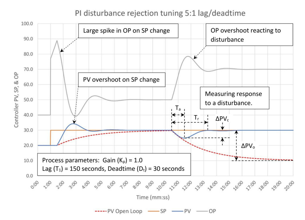
Figure 1: PI controller tuned for disturbance rejection. Tuning constants are K = 3.655, Ti = 1.53 minutes/repeat, Td = 0 minutes. Courtesy: Ed Bullerdiek, retired control engineer
Ideally disturbance rejection tuning should produce a symmetrical process variable (PV) curve as the controller corrects the disturbance (starting at the 10:30 mark in Figure 1), however, my personal preference to avoid secondary oscillations requires leaving the integral just a little slow. You may choose to speed up the integral and increase gain to get the desired shape, but this will cause secondary oscillations.
There are three performance measures for disturbance rejection tuning:
- Arrest time (Ta): The time to stop the process variable movement away from setpoint after a disturbance starts.
- Recovery time (Tr): The time when the process variable returns to setpoint. Minor oscillations can be ignored, however large oscillations should be included in the recovery time.
- Disturbance rejection effectiveness: Effectiveness is calculated from the difference in the open (ΔPVo) and closed (ΔPVc) loop response of the process. To express this percentage, the calculation is:
| Eff = | 100 * | (ΔPVo – ΔPVc) |
| ΔPVo |
Arrest time is mostly affected by deadtime (Dt) followed by the process lag (T1). Recovery time is also affected by integral tuning. Disturbance rejection effectiveness is a function of the lag/deadtime ratio; the higher the ratio the more effective disturbance rejection will be. Disturbance rejection effectiveness can exceed 98% for a 100:1 lag/deadtime ratio. It’s closer to 85% for a 10:1 ratio and just 74% at a 5:1 ratio. Effectiveness drops below 1% at ratios lower than 1:4.
There are tradeoffs when you employ PI disturbance rejection tuning. From Figure 1 these are:
- On a setpoint (SP) change there will be a large spike in the controller output (OP) and the process variable (PV) will overshoot the setpoint. How badly depends on the lag/deadtime ratio; the higher the ratio the worse the OP spike and PV overshoot will be.
- When a disturbance occurs the OP will overshoot its final value by 50% to 75% depending on ratio.
The first problem is by far the worst for lag dominant processes, but it is the easiest to solve if you have access to almost any kind of setpoint management options or have access to the integral-only on setpoint change PID algorithm. Managing controller output overshoot requires slowing down the integral, which defeats the purpose of disturbance rejection tuning.
Proportional-integral-derivative (PID) disturbance rejection tuning:
Figure 2 displays the performance enhancement we can achieve if we use derivative for proportional-integral-derivative (PID) disturbance rejection tuning.
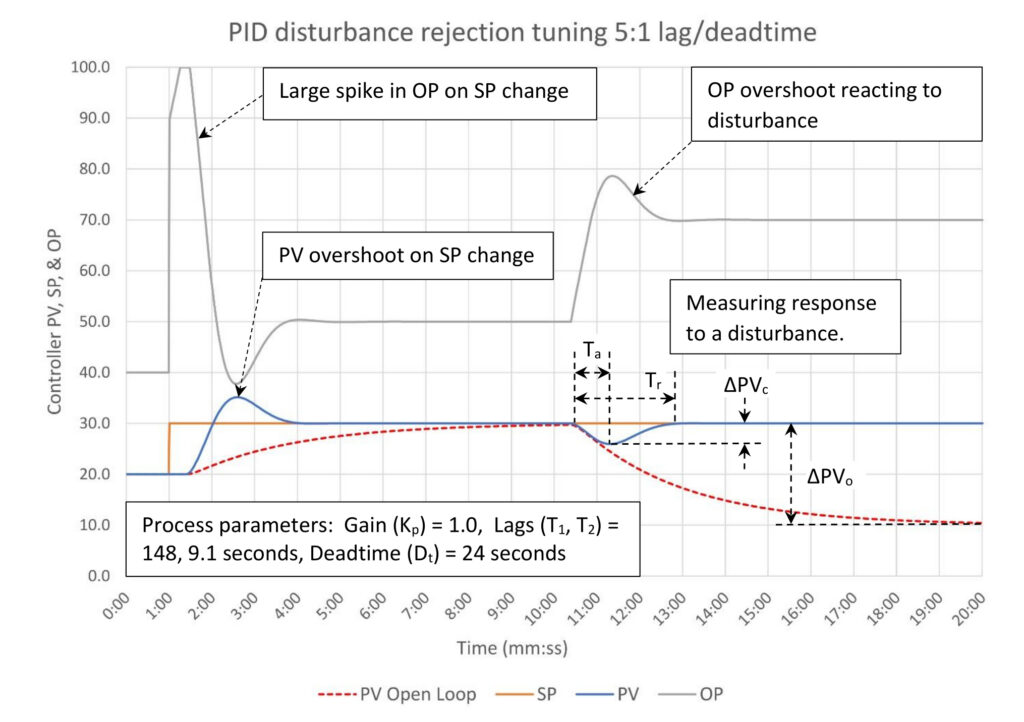
Figure 2: PID controller tuned for disturbance rejection. Tuning constants are K = 4.9, Ti = 1.2 minutes/repeat, Td = 0.18 minutes. Courtesy: Ed Bullerdiek, retired control engineer
First note that this is not a true first order plus deadtime (FO+Dt) process. You cannot use derivative on a true FO+Dt process because derivative behaves badly on sudden changes in direction. Adding a second lag smooths the process’s change of direction, which takes the spikes out of the derivative response. Regardless, this process has a deadtime of 30 seconds and a lag of 150 seconds as measured by an open loop step test. Fortunately, there are very few true FO+Dt processes in the real world, therefore we can generally assume that we can use derivative.
Adding derivative allows us to use more controller gain and faster integral, which results in better overall performance (Table). As expected, this improved disturbance rejection efficiency and sped up overall response.

Of course, the tradeoffs are also made worse. The controller output spike is even bigger; in this case it saturates at 100% output for a short period. The rate of change of the controller output is also faster (as it must be to shorten arrest and recovery time), however the percentage of overshoot doesn’t change much.
Mapping disturbance rejection tuning
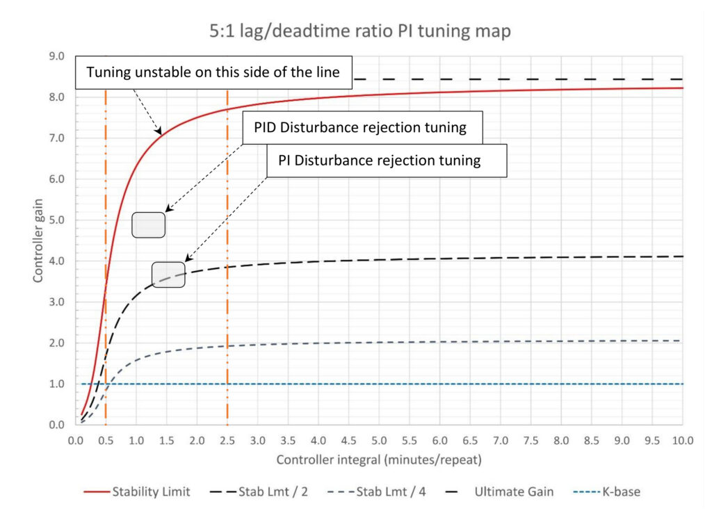
Figure 3: Self-limiting process PI controller tuning map. Lag/deadtime ratio = 5:1. Kp = 1.0, T1 = 150 seconds, Dt = 30 seconds. Courtesy: Ed Bullerdiek, retired control engineer
Figure 3 is the proportional-integral (PI) controller tuning map for this process with the two disturbance rejection windows plotted on it. This map will be used to help us visualize where each of the controller tuning windows exists relative to stability limits, deadtime and the process lag. Working from the top the horizontal lines are:
- The top dashed line just above the controller gain of 8 is the ultimate gain (Ku = 8.44) for this process.
- The solid line marked “stability limit” is the maximum combination of controller gain and integral that are stable for this process. All gain and integral settings below and to the right of this line are stable. This doesn’t mean that all of them are good for control…
- The “stab lmt/2” line roughly delimits where oscillations begin for PI controllers (do not use derivative). We should generally avoid PI tuning constant combinations much above or to the left of this line unless we add derivative.
- The “stab lmt/4” line roughly delimits where critically damped controller response occurs.
- The “K-base” line is the baseline controller gain (Kbase) for this process (Kbase = ΔOP/ΔPV).
Not surprisingly, the PI disturbance rejection tuning window is at the tightest corner of the curve in the stability limit/2 line (where the gain starts to drop as the integral gets faster). The window does cover part of the region above the curve where we can expect some oscillations in the controller response. The top left corner of the window (K = 4.0, Ti = 1.25) does have a symmetrical PV response to a disturbance, but at the cost of some swinging after the initial response.
The PID disturbance rejection window is well into the region where we would expect oscillations if derivative weren’t applied. Note how close the window is to the stability limit. There is considerable risk in tuning this close to stability limits; any change in the process that (for example) increases deadtime will push the tuning into instability (be careful about noise filters).
Note also that for this process the PI disturbance rejection tuning window is midway between the deadtime and process lag time (orange vertical lines at 0.5 and 2.5 minutes). This window will move as the lag/deadtime ratio changes, tending to stay closer to deadtime than lag time as the ratio increases. Similarly the PID disturbance rejection tuning window while closer to the deadtime line also will move as the lag/deadtime ratio changes.
What is critically damped/setpoint following tuning?
Critically damped tuning is used where we expect that we will be changing the SP of a controller frequently. Our goal is to get the PV to the new SP as fast as possible without PV overshoot and the oscillation that follows (critically damped response). Figure 4 is the same process used in Figure 1 but tuned for critically damped response.
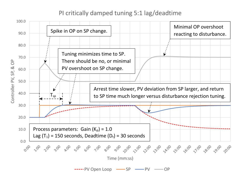
Figure 4: PI controller with critically damped tuning. Tuning constants are K = 2.03, Ti = 2.10 minutes/repeat, Td = 0 minutes. Courtesy: Ed Bullerdiek, retired control engineer
“As fast as possible” implies that the controller should be able to get the process variable (PV) to the new setpoint (SP) faster than open loop response, and we can see in figure 4 that the PV gets to the SP in a little more than 2 minutes. The open loop response (dashed line) shows that the PV does not reach the SP by the time the disturbance shows up, or after more than nine and one-half minutes. In reality, how much faster depends on the lag/deadtime ratio; the higher the ratio the faster the controller can get the PV to the new SP.
But there is a tradeoff for getting the PV to SP faster; the controller output (OP) must spike above its final resting value. At higher lag/deadtime ratios the OP spike can be excessive. If this will cause problems elsewhere in the process you may need to further slow the controller tuning, but this would forego the additional benefit of critically damped tuning.
Critically damped tuning also minimizes OP overshoot when a disturbance occurs. We can think of this as “fastest possible response to disturbances without OP overshoot,” which is a fancy way of saying we want it fixed fast – but not too fast. Relative to disturbance rejection tuning the disturbance arrest time is longer and disturbance rejection effectiveness is poorer, but not that much. The real problem occurs with disturbance recovery time. With disturbance rejection tuning the recovery time is between two and three times longer than the arrest time. With critically damped tuning recovery time can be many multiples of arrest time and the higher the lag/deadtime ratio the worse it is.
There is one additional performance measure for critically damped tuning: process variable time to setpoint following a setpoint change (Tsp). Small changes in tuning can have a big impact on this. To get consistent measurements during the development of data for these articles critically damped tuning was set to have 5% PV overshoot (a 10% setpoint change resulted in 10.5% total PV movement before the PV returned to SP. Tsp is the time to when PV crosses SP.) Of course, the disturbance rejection performance measures are still relevant.
Mapping critically damped tuning
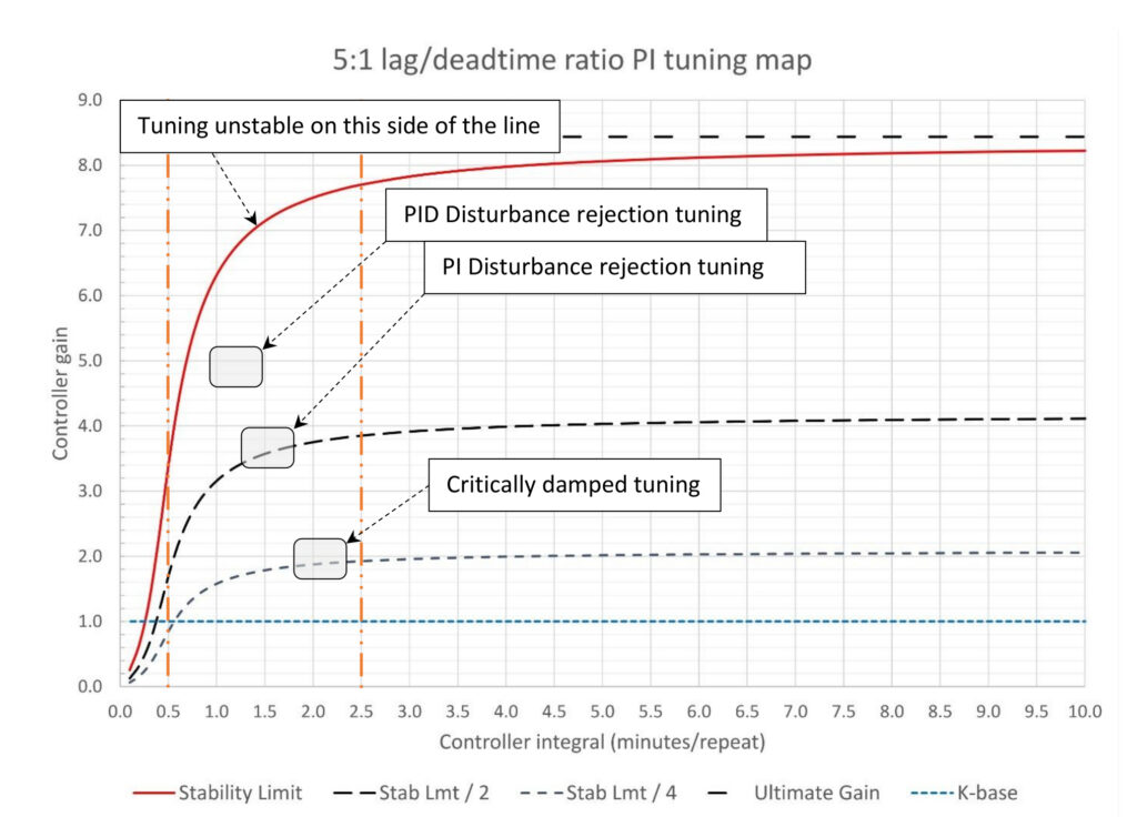
Figure 5: Self-limiting process PI controller tuning map. Lag/deadtime ratio = 5:1. Kp = 1.0, T1 = 150 seconds, Dt = 30 seconds. Courtesy: Ed Bullerdiek, retired control engineer
In Figure 5 the critically damped tuning window has been added to the PI controller tuning map. It is close to the stability limit /4 line as noted above and it is somewhat to the left (faster than) the process lag. This window also moves as the lag/deadtime ratio changes, floating between the deadtime and lag time constants as the ratio increases. Interestingly the integral constant for critically damped tuning is faster than for disturbance rejection tuning at low lag/deadtime ratios.
What is minimum output movement tuning?
Your first question is why would I tune for minimum output movement? After all no textbook or loop tuning guide discusses this. It does seem counterintuitive to tune a controller to do almost nothing.
The first answer is minimum output movement tuning is the only tuning that will work for deadtime dominant processes. Once the lag/deadtime ratio drops below 1:4 nothing else works and it may be your preferred tuning on processes up to a 1:1 lag/deadtime ratio. The second answer is minimum output movement tuning is the highest controller gain/fastest integral corner of the slow optimization tuning window. Knowing where this might be may help you set up slow optimization tuning that doesn’t impact the rest of the process.

Figure 6: PI controller tuned for minimum OP movement. Tuning constants are K = 0.8238, Ti = 2.571 minutes/repeat, Td = 0 minutes. Courtesy: Ed Bullerdiek, retired control engineer
Figure 6 is the same process used in figures 1, 2 and 4 tuned for minimum output movement. Controller response to a setpoint change looks nearly like an operator changing the controller output. There is a slight corner cut off where the tuning matches the final output when the process variable starts moving. This results in the PV following the open loop response path. During the controller response to a disturbance, the controller output mirrors the PV open loop response curve (multiplied by the inverse of the process gain. In this example the process gain is 1.0 which yields a perfect mirror.)
There are no additional performance measurements for minimum output movement tuning. There should be no controller output movement once the process variable starts moving after a setpoint change. The goal is to let any other part of the process that is affected by the output movement to respond without further disturbance from this controller. We are still concerned about disturbance rejection but have determined that eliminating the disturbance takes a back seat to other process priorities. Obviously slow tuning slows disturbance arrest time, lowers disturbance rejection and considerably extends the time to eliminate the disturbance.
Mapping minimum controller output movement tuning
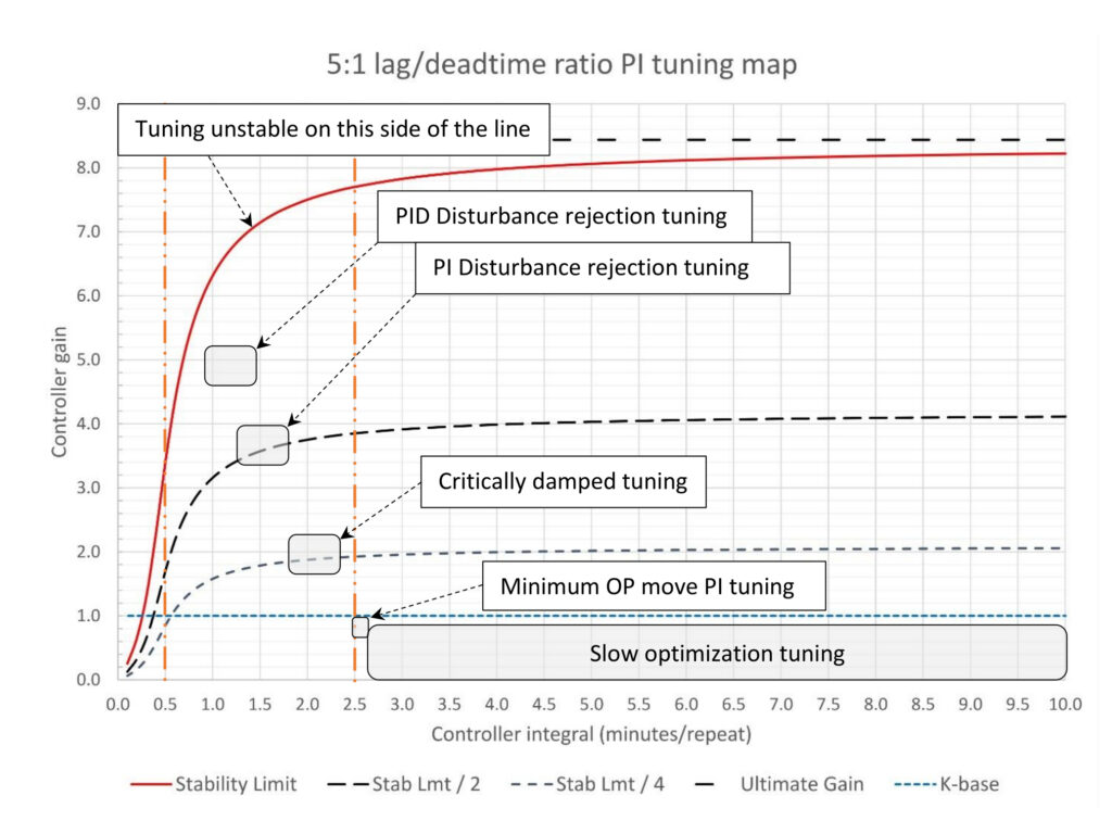
Figure 7: Self-limiting process PI controller tuning map. Lag/deadtime ratio = 5:1. Kp = 1.0, T1 = 150 seconds, Dt = 30 seconds. Courtesy: Ed Bullerdiek, retired control engineer
The minimum controller output movement and slow optimization tuning windows have been added to the PI tuning map in Figure 7. The minimum controller output movement window will always be just below the baseline controller gain (Kbase), which, in this case, is slightly below 1.0 (Kbase is the inverse of the process gain) and the integral will always be larger than the process lag. As the lag/deadtime ratio falls the controller gain becomes smaller relative to Kbase and the integral constant grows larger relative to the process lag.
What is slow optimization tuning?
Process controllers can be ranked based on their purpose, starting with controllers that have safety consequences. For example we don’t ever want fuel gas pressure to get so low that we trip heaters on low fuel gas pressure. After this comes controllers that affect equipment interlocks and then basic regulatory controls. Then we need to think about system control objectives. For starters we are very interested in controlling the quality of the products that we sell; these will get closed loop controls.
After this there are internal streams or low value products whose composition could be controlled but often aren’t, typically because it is thought that controlling them will interfere with regulatory controllers or more important product qualities. There are also a number of opportunities to push the process in more economic directions or make moves to extend equipment life. All of these tend to be slow and yes, aggressively controlling these will interfere with more important controls.
The traditional approach to all these opportunities in refining was to leave it up to the operators. Does controlling the bottom product quality on a distillation tower affect the overhead product quality? Yes? Then let the operator worry about it. This has changed in recent years and multivariable model-based control has become the standard answer.
However, if you cannot afford or do not have the technical acumen to install model-based controls or if you only have a couple of these types of control opportunities, PID control can still be used. There is a general rule that says slow moving controllers can’t upset fast controllers.
How do I pick a tuning method (when it’s easy)?
One of the themes of this series is that using only one loop tuning method is not likely to get you the result you are looking for. Most tuning methods give you one set of tuning constants that supposedly are the perfect solution for your problem. Based on the foregoing this is self-evidently not true. So how well do some common methods work?
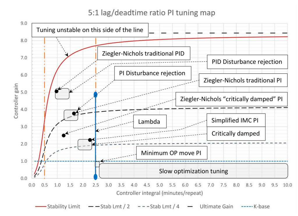
Figure 8: Self-limiting process PI controller tuning map. Lag/deadtime ratio = 5:1. Kp = 1.0, T1 = 150 seconds, Dt = 30 seconds. Courtesy: Ed Bullerdiek, retired control engineer
Five tuning methods have been added to the 5:1 lag/deadtime ratio PI tuning map in Figure 8. As it turns out for this lag/deadtime ratio traditional Ziegler-Nichols (Z-N) PID and PI tuning each land in the PID and PI disturbance rejection windows and simplified IMC PI tuning lands on the edge of the critically damped tuning window. Lambda tuning, which is a dial-a-response method, is the blue line at the 2.5 minutes/repeat integral line that stretches from a controller gain of zero to five. It passes close to the critically damped window and the minimum output movement window. The Z-N critically damped calculations miss all the windows.
In summary, for this process all five tuning methods will deliver reasonable results as long as you know which one to select for the performance you need. However, a 5:1 lag/deadtime ratio process is not hard to tune because its stability limit is far above the baseline controller gain (Kbase). Even minimum output movement tuning will get you 55% disturbance rejection effectiveness. In this case, you are aiming at a very large target.
How do I pick a tuning method (when it’s hard)?
In PID spotlight part 6, we learned that as lag/deadtime ratio drops tuning becomes more difficult. In fact, deadtime dominant processes are very hard to tune effectively, and even when we get it right disturbances are still fully expressed and persistent.
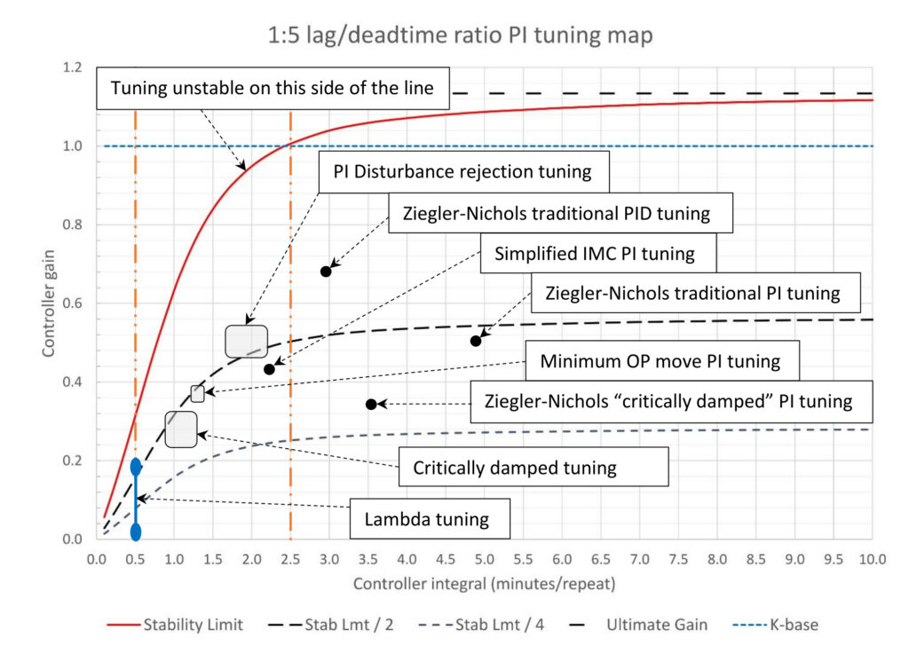
Figure 9: Self-limiting process PI controller tuning map. Lag/deadtime ratio = 1:5. Kp = 1.0, T1 = 30 seconds, Dt = 150 seconds. Courtesy: Ed Bullerdiek, retired control engineer
Figure 9 is the PI tuning map for a deadtime-dominant process with a 1:5 lag/deadtime ratio. The lag is now 0.5 minutes and the deadtime 2.5 minutes, which makes this process the inverse (if such can be said) of the 5:1 L/D ratio process above. The first thing that should stick out is the ultimate controller gain (Ku) at 1.134 is only now marginally higher than the baseline controller gain (Kbase). This tells us that our tuning window is compressed and getting reasonable tuning will be difficult.
The next thing to note is how the PI disturbance rejection, critically damped and minimum output movement tuning windows have moved around relative to each other, with the disturbance rejection integral remaining close to the process deadtime and critically damped integral remaining close to the process lag. (PID disturbance rejection tuning is not possible at this lag/deadtime ratio.) In reality, we are at a point where PI disturbance rejection tuning makes no sense as the best rejection effectiveness is now down to 0.6%. No matter what we do, a disturbance will be 99.4% expressed. The best we can do is eliminate the disturbance cleanly once the deadtime has passed, which PI disturbance rejection tuning doesn’t do.
We are also at a point where critically damped tuning ceases to make sense either. Controller gain is too small and integral is too fast, which results in process variable overshoot and small swings that take some time to finally settle out.
Minimum controller output movement tuning works very well, but this is expected as it is intended specifically for use on deadtime dominant processes.
Of the five loop tuning methods shown, only the simplified IMC method resulted in reasonable tuning constants. The integral is too slow, which will result in slow process variable recovery to setpoint after a disturbance. This can be trimmed out using heuristic methods (see PID spotlight part 10). For background the simplified IMC method was specifically designed to give reasonable results for all lag/deadtime ratios between 100:1 and 1:100. At high ratios the controller gain is limited to manage problems with large controller output spikes on a setpoint change (giving up on disturbance rejection effectiveness), and it trends toward critically damped through moderate lag/deadtime ratios.
The Z-N methods shown give very poor results. The traditional Z-N PID tuning is borderline unstable, primarily because derivative cannot be used on deadtime dominant processes. The other two Z-N methods set integral too slow, however they are at least stable. Lambda tuning sets integral far too fast, which will result in oscillations for any reasonable controller gain setting. None of these methods should be used to calculate tuning constants for a deadtime dominant process. None of this should be surprising given how far the results of all these methods are from the tuning windows.
Can I predict where my controller tuning window is?
Once you have decided how aggressive you want your PID controller to be you need to predict where the controller tuning window is. It also wouldn’t hurt to be able to predict performance (although in practice we will tune for the best that we can get and if it isn’t good enough work on alternative methods to get better results). The in-depth discussion of these two topics will be done in the next two articles, but the following two figures will offer a glimpse at what is coming.
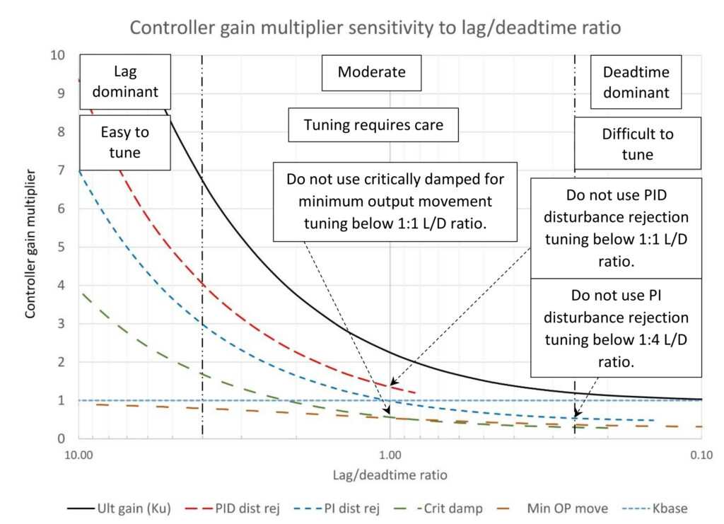
Figure 10: Map of baseline controller gain (Kbase) multipliers for PID and PI disturbance rejection, critically damped and minimum OP movement tuning based on lag/deadtime ratio for self-limiting processes. Courtesy: Ed Bullerdiek, retired control engineer
Figure 10 is the grown-up version of Figure 1 in PID spotlight part 6 shortened to focus on the range of lag/deadtime ratios between 10:1 and 1:10, which is where all the interesting changes happen. There is a new set of lines on this chart:
- Ultimate controller gain (Ku)
- PID disturbance rejection controller gain (= 0.6 * Ku)
- PI disturbance rejection controller gain (= 0.45 * Ku)
- Critically damped controller gain (= 0.25 * Ku)
- Minimum output movement controller gain
- Baseline controller gain (Kbase)
The Ziegler-Nichols method for estimating controller gain works very well and is used for predicting PI and PID disturbance rejection and critically damped controller gain. (Z-N does not work well for predicting integral constants across most lag/deadtime ratios).
As the lag/deadtime ratio drops, there are three events of note:
- Below a lag/deadtime (L/D) ratio of 1:1 critically damped tuning controller gain drops below minimum controller output movement gain. Below this point, critically damped tuning should not be used, opting for minimum controller output movement instead.
- PID disturbance rejection tuning should not be used on deadtime dominant processes (L/D ratios less than 1:1).
- PI disturbance rejection tuning should not be used on deadtime dominant processes with L/D ratios less than 1:4.
Can I predict how effective my controller will be?
As stated above there are multiple measures of controller effectiveness. The one we are usually most interested in is disturbance rejection effectiveness. We want our process to be on setpoint.
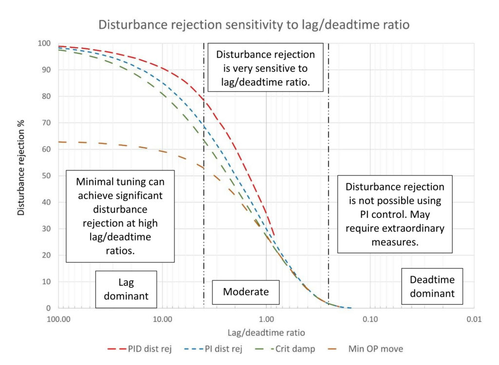
Figure 11 plots disturbance rejection effectiveness for PID and PI disturbance rejection, critically damped, and minimum controller output movement tuning. What’s interesting here is how rapidly disturbance rejection effectiveness drops between the 4:1 and 1:4 lag/deadtime ratios, the moderate lag/deadtime ratio band. This points up the critical importance of avoiding anything that artificially increases deadtime, for example adding excessive filtering to attenuate a noisy signal.
The next thing to note is that PID disturbance rejection tuning can improve disturbance rejection effectiveness better than 10% in the upper part of the moderate process band (4:1 to 1:1 lag/deadtime ratio) and better than 5% at a 10:1 lag/deadtime ratio. If maximum disturbance rejection is required then including derivative should be strongly considered.
Finally, there does not appear to be that big of a disturbance rejection performance gap between PI disturbance rejection tuning and critically damped tuning. This is a little misleading. There is a large gap in recovery time after a disturbance between these two tuning styles (PI disturbance rejection tuning and critically damped tuning). There are multiple performance measures we need to keep in mind, which we will discuss when we dig into performance measures.
What if I need more performance?
Finally, we need to talk about extraordinary measures. You will need to deploy extraordinary measures when a simple PID controller cannot deliver the performance you need, especially if you are working with a deadtime dominant process. This doesn’t mean that you cannot use PID control. It means that you can only achieve the performance you require through a combination of design decisions, advanced PID controller features, feedforward and/or external logic to squeeze that additional performance out of your PID controller. These extraordinary measures will be the subject of future articles.
A quick recap of tuning for purpose
A proportional-integral-derivative controller rarely exists in a vacuum. When it acts the changing controller output affects other parts of the process. The first decision you must make is how to weigh the importance of keeping the controller’s process variable on setpoint versus how well the rest of the process can tolerate controller output movement. The options are:
- Disturbance rejection: Keeping the process variable on setpoint is far more important than any impact the controller output movement has on the rest of the process.
- Critically damped: Keeping the process variable on setpoint has equal weight to the impact of controller output movement on the rest of the process.
- Slow optimization: Minimizing controller output movement is required to avoid impacting the rest of the process while still maintaining some control over the process variable.
These three general goals exist on a continuum, and the proper tuning for any specific PID controller can be anywhere from the most aggressive full PID disturbance rejection tuning to extremely slow optimization.
Ed Bullerdiek is a retired control engineer with 37 years of process control experience in petroleum refining and oil production. Send comments and questions to [email protected]. Edited by Mark T. Hoske, editor-in-chief, Control Engineering, WTWH Media, [email protected].
Keywords
Proportional-integral-derivative, PID tutorial
Learning objectives
- Understand that processes may be very complex and that a PID controller should be tuned fast to eliminate disturbances, slow to avoid disturbing the rest of the process or perhaps in between to balance competing goals.
- Know the five PID controller tuning performance windows, including what they do well and the tradeoffs of each window.
- Know the industrially relevant performance measures for PID controllers.
- Understand that various common tuning methods may not yield good results depending on controller performance goals and lag/deadtime ratio.
Consider this
A PID controller rarely exists in a vacuum. Understanding the PID controller’s role in the entire process will allow you to select a performance goal that will optimize the entire process’s performance.
You also might like
PID series from Ed Bullerdiek, retired control engineer
PID Spotlight, part 1: Three reasons to tune control loops: Safety, profit, energy efficiency
PID spotlight, part 2: Know these 13 terms, interactions
PID spotlight, part 3: How to select one of four process responses
PID spotlight, part 4: How to balance PID control for a self-limiting process
PID spotlight, part 5: What does good and bad controller tuning look like?
PID spotlight, part 6: Deadtime? How to boost controller performance anyway
PID spotlight, part 7: Open-loop tuning of a self-limiting process
PID spotlight, part 8: Closed-loop tuning for self-limiting processes
PID spotlight, part 9: Heuristic tuning for a self-limiting process (part A on heuristic tuning)
PID spotlight, part 10: Heuristic tuning in a self-limiting process
PID spotlight, part 11: How a PID controller works with an integrating process
PID spotlight, part 12: What does good and bad controller tuning look like?
PID spotlight, part 13: Deadtime: what’s the best that I can do?
PID spotlight, part 14: Open loop tuning of an integrating process
PID spotlight, part 15: Open loop tuning of near integrating processes
PID spotlight, part 16: Closed loop tuning of an integrating process
PID spotlight, part 17: Heuristic tuning of an integrating processes
PID spotlight, part 18: Identifying control valve performance problems
PID spotlight, part 19: PID controller tuning mechanics
PID spotlight, part 20: Tuning with bad valves
PID spotlight, part 21: Noise: Can I tune around it?
PID spotlight, part 22: Can I tune a noisy PID controller?
PID spotlight, part 23: Filtering noise for better PID control
PID spotlight: part 24: How do I tune PID controllers during a new unit startup?
PID spotlight, part 25: Navigating PID controller tuning
More on PID and advanced process control from Control Engineering