You need aggressive control to manage disturbances, but when you change setpoint the control response upsets the process. How can you shape the controller response to meet your needs?
Insights about shaping controller response
- Aggressive PID controller tuning of lag dominant self-limiting processes can result in excessive controller output movement after a setpoint change. Users will often slow controller tuning to mitigate this movement, resulting in reduced controller performance.
- The use of setpoint ramps, setpoint filters or the integral only on setpoint change algorithm can greatly reduce the excess controller output movement problem.
- Controller tuning and the tuning of a feature work together to shape the controller response, allowing you to form the controller response you need. Setpoint ramps and filters can help.
Tuning proportional-integral-derivative (PID) controllers requires that we make tradeoffs. In the case of a lag dominant process the tradeoff is between the controller response to disturbances and controller output movement, especially after setpoint changes.
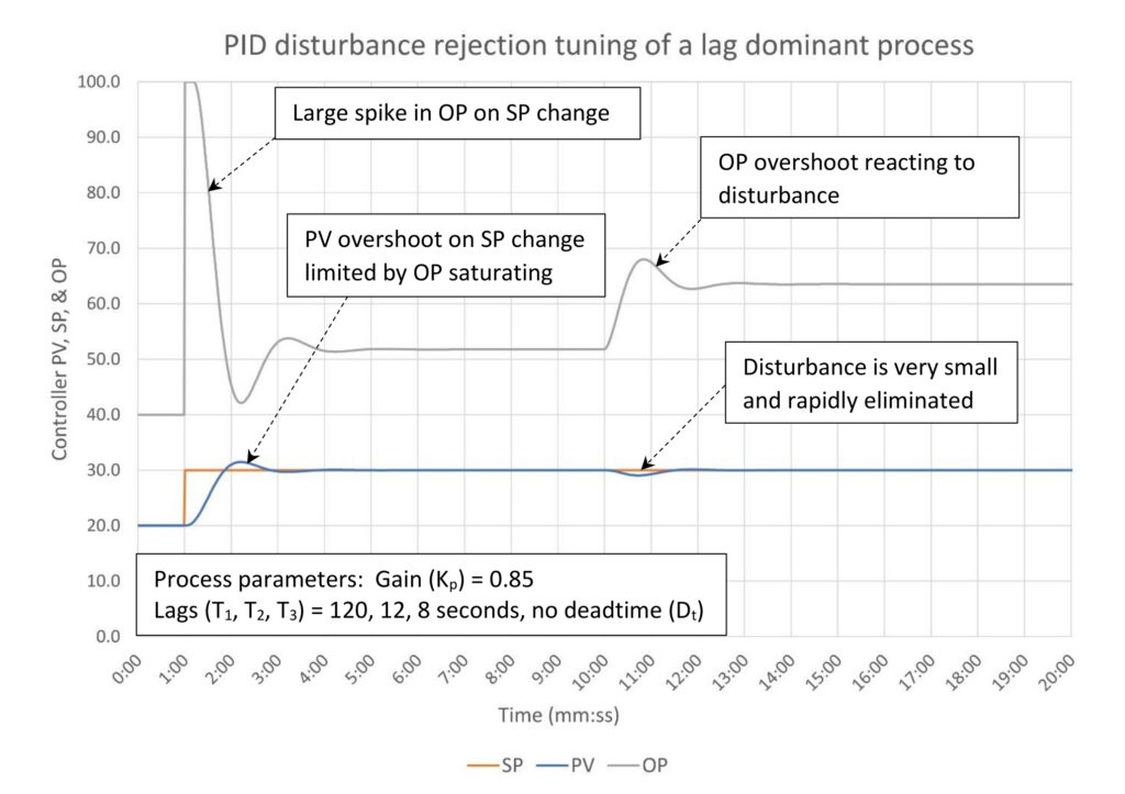
Figure 1: PID controller tuned for disturbance rejection (9.2:1 lag/deadtime ratio). Tuning constants are K = 10.4, Ti = 0.62 minutes/repeat, Td = 0.12 minutes. Courtesy: Ed Bullerdiek, retired control engineer
Figure 1 displays the dilemma facing us. Disturbance rejection tuning does exactly what it is designed to do; the disturbance is very small and rapidly eliminated. However, a controller gain of 10 causes a large spike of controller output (OP) whenever the setpoint (SP) is changed. We would normally expect to see the process variable (PV) considerably overshoot the new setpoint, but in this case the controller output saturates, which limits the overshoot. If large rapid changes in the controller output can upset other parts of the process we have a potential problem.
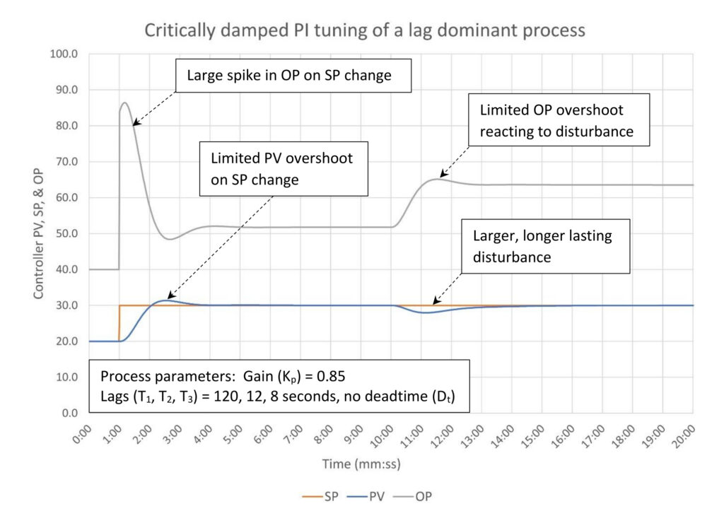
Figure 2: PID controller tuned for critically damped response (9.2:1 lag/deadtime ratio). Tuning constants are K = 4.345, Ti = 1.635 minutes/repeat, Td = 0 minutes. Courtesy: Ed Bullerdiek, retired control engineer
One solution, of course, is to slow down the controller tuning. Figure 2 shows the same process with the controller response set to critically damped tuning. The controller output overshoot after a setpoint change is reduced but still substantial. Slower tuning results in a larger and longer lasting disturbance. If the controller output spike is still too large, we could continue to reduce the controller gain, but at the cost of still larger and longer lasting disturbances. Let’s explore how using advanced PID controller features can offer a better approach.
Advanced PID controller features
We can address the controller output spike problem by using a:
- Setpoint ramp
- Setpoint filter
- Integral only on setpoint change PID algorithm
These features are available in some control systems, or the first two often can be added through programming. If any of these features are available in your system, please note that there are no industry standards regarding how these features should work. Before applying these features, you should perform tests to see exactly how they work.
Setpoint ramp purpose, application example
A setpoint ramp slowly moves the setpoint of a controller from one value to another at a fixed rate. Depending on the system you either enter a ramp rate (Δ%/minute) or the time for the setpoint to get to its final value.
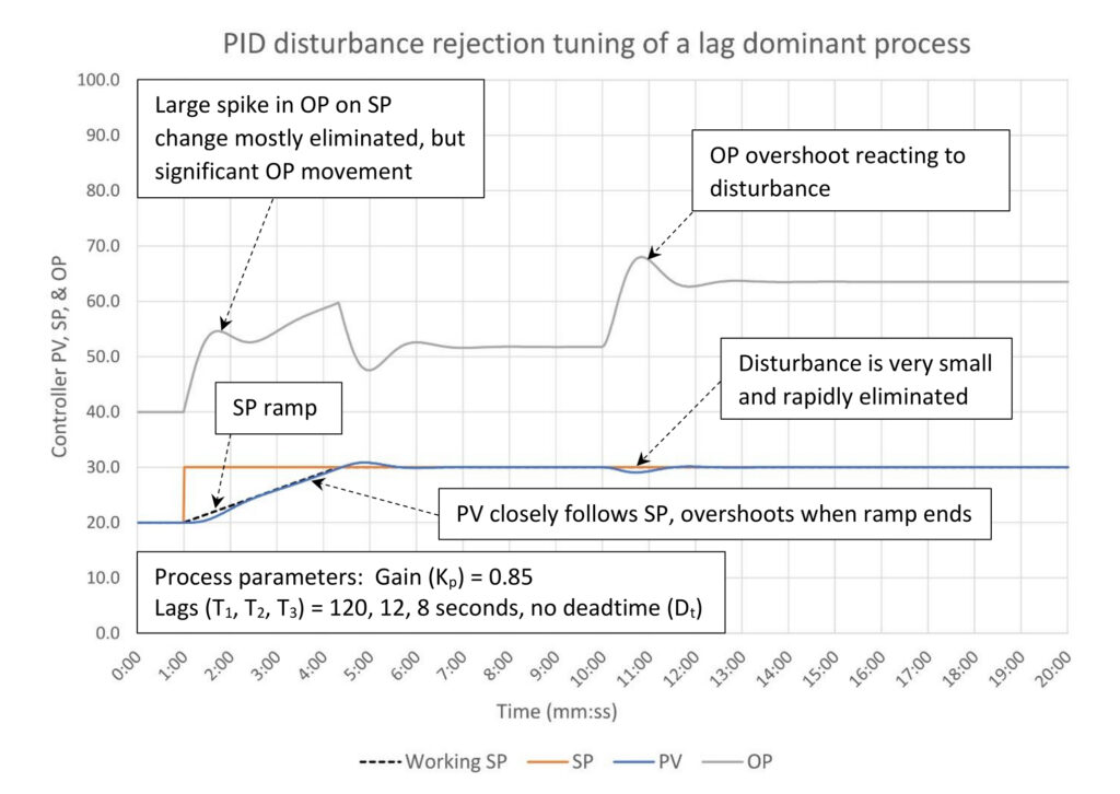
Figure 3: PID controller tuned for disturbance rejection (9.2:1 lag/deadtime ratio). Tuning constants are K = 10.4, Ti = 0.62 minutes/repeat, Td = 0.12 minutes. SP ramp rate is 3%/minute. Courtesy: Ed Bullerdiek, retired control engineer
In Figure 3 a setpoint ramp has been added to the PID disturbance rejection tuning of this process. In this system, the setpoint ramp is programmed as a rate and displayed as a “working setpoint.” The disturbance is still small and rapidly eliminated, but the large controller output (OP) spike that normally follows a setpoint change has been considerably reduced.
There is, however, still a good bit of controller output movement as the controller tries to keep the PV on setpoint (SP) during the ramp. Most of the movement occurs at the start of the ramp when the controller is responding to the gap between PV and SP caused by deadtime and the end of the ramp when the PV overshoots the SP because of deadtime. One way to manage this movement is by slowing down the ramp rate, but the tradeoff is it takes longer to get to setpoint. You may have to experiment with ramp rate to get to an optimal balance.
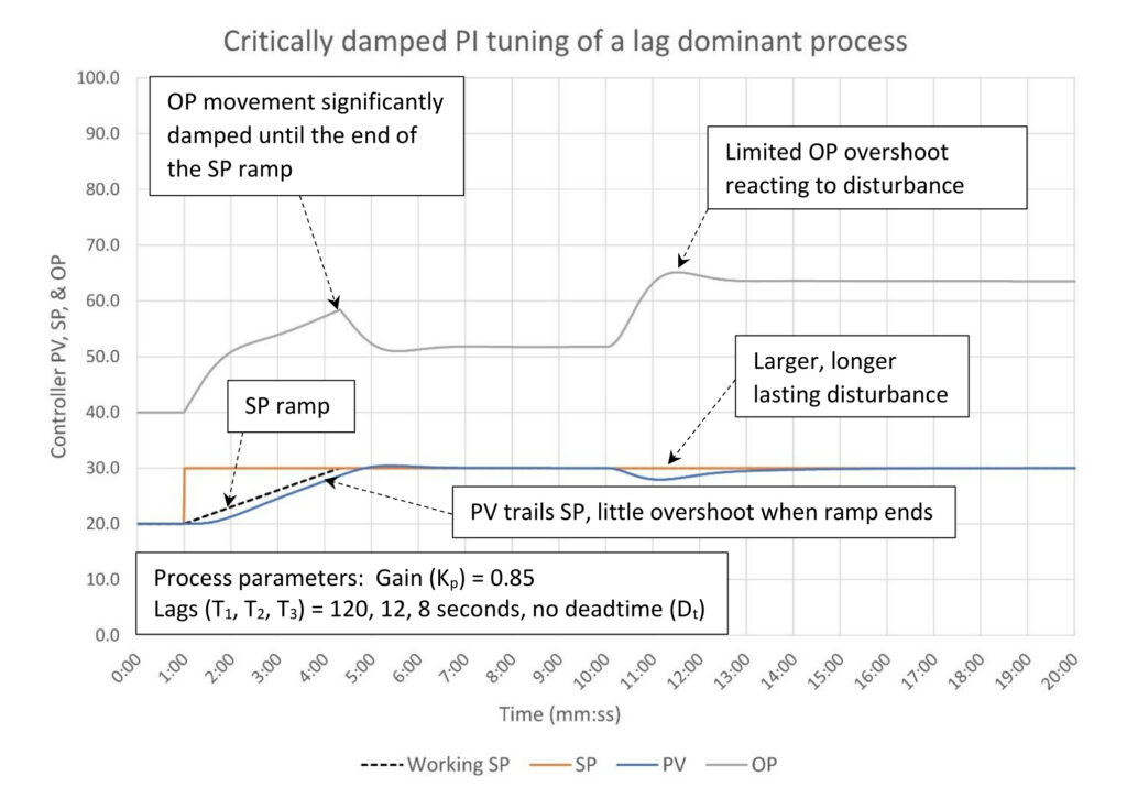
Figure 4: PID controller tuned for critically damped response (9.2:1 lag/deadtime ratio). Tuning constants are K = 4.345, Ti = 1.635 minutes/repeat, Td = 0 minutes. SP ramp rate is 3%/minute. Courtesy: Ed Bullerdiek, retired control engineer
If the controller output movement is still excessive, we can combine the SP ramp with slower controller tuning (Figure 4). Slowing down the tuning causes the process variable to trail the setpoint ramp, which isn’t a problem, and it has very little overshoot of the setpoint when the ramp ends. Controller output movement is relatively restrained with the exception of a sharp change in direction when the ramp ends, which is unavoidable. If you need faster PV response to a SP change you can increase the SP ramp rate; a 5%/minute ramp rate still has acceptable response (in my opinion).
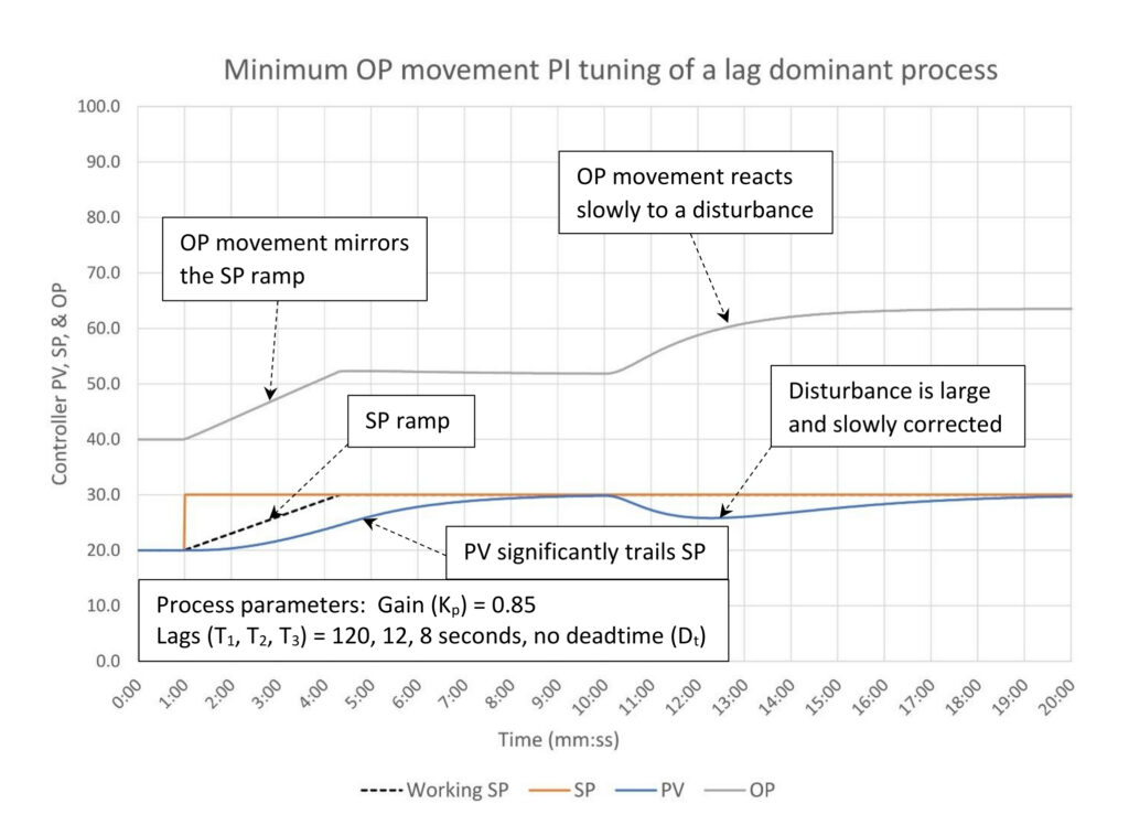
Figure 5: PID controller tuned for minimum output movement response (9.2:1 lag/deadtime ratio). Tuning constants are K = 1.049, Ti = 1.877 minutes/repeat, Td = 0 minutes. SP ramp rate is 3%/minute. Courtesy: Ed Bullerdiek, retired control engineer
Finally, the last word in slowing down controller tuning is shown in figure 5. Minimum controller output (OP) movement tuning would only be used on a lag dominant process if the controller is intended for slow optimization. It would make sense to add a setpoint ramp to dampen controller output movement when the setpoint is changed. When setpoint ramping is used the OP mirrors the setpoint ramp. The process variable will considerably trail the setpoint ramp, but this shouldn’t be a concern. Otherwise, controller performance is what we would expect from a controller tuned this slow; when a disturbance occurs output movement is slow, the process variable is allowed to move relatively far from setpoint, and it takes considerable time for the controller to eliminate the disturbance.
Setpoint filter use and settings
A setpoint filter feeds a setpoint change to the PID controller through a first order filter. Normal guidance is the setpoint filter should equal the process lag constant identified in an open-loop step test, but there is room for adjustment. If open-loop step test data is not available, set the setpoint filter equal to about four times the integral constant if you are using disturbance rejection tuning (PID or PI) or two times the integral constant if you are using critically damped tuning. This is approximate; you may need to adjust the filter time until you are happy with the results.

Figure 6: PID controller tuned for disturbance rejection (9.2:1 lag/deadtime ratio). Tuning constants are K = 10.4, Ti = 0.62 minutes/repeat, Td = 0.12 minutes. SP filter rate is 2.1 minutes. Courtesy: Ed Bullerdiek, retired control engineer
Figure 6 shows the response of a PID controller tuned for disturbance rejection with a setpoint (SP) filter set equal to the process lag (T1 = 2.1 minutes). The process variable (PV) closely follows the SP filter (working SP line). The controller output (OP) overshoots its final value after a SP change about the same amount it overshoots the final OP after an equivalent disturbance. This would seem to be a reasonable tradeoff, however, there is some room to work with this. For example, a natural question to ask is if some SP filtering is good, could more filtering be better?
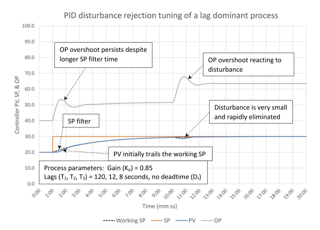
Figure 7: PID controller tuned for disturbance rejection (9.2:1 lag/deadtime ratio). Tuning constants are K = 10.4, Ti = 0.62 minutes/repeat, Td = 0.12 minutes. SP filter rate is 3.15 minutes. Courtesy: Ed Bullerdiek, retired control engineer
In figure 7 we’ve increased the SP filter time 50% to 3.15 minutes. The initial controller output (OP) overshoot is somewhat smaller but remains. The overshoot occurs because the process deadtime allows a gap to grow between the setpoint and the process variable, which the aggressive tuning then works to eliminate. And, of course, the time for the PV to get to setpoint is extended. Increasing the SP filter will never fully eliminate the OP overshoot on a SP change for a controller that is tuned for disturbance rejection. If controller output overshoot is really objectionable, then controller tuning must be slowed down.
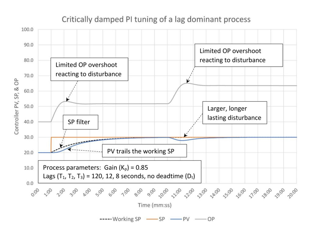
Figure 8: PID controller tuned for critically damped response (9.2:1 lag/deadtime ratio). Tuning constants are K = 4.345, Ti = 1.635 minutes/repeat, Td = 0 minutes. SP filter rate is 2.1 minutes. Courtesy: Ed Bullerdiek, retired control engineer
As seen in figure 8 critically damped tuning combined with a setpoint filter can largely eliminate controller output (OP) overshoot. The particular example shown in figure 8 is tuned slightly faster than critically damped, which leaves some OP overshoot after both the setpoint change and the disturbance. Slowing down the SP filter to 3.15 minutes does eliminate the OP overshoot after the SP change. Note that the PV does follow the working SP, but not as closely as it would with disturbance rejection tuning due to the slower controller tuning.

Figure 9: PID controller tuned for critically damped response (9.2:1 lag/deadtime ratio). Tuning constants are K = 4.345, Ti = 1.635 minutes/repeat, Td = 0 minutes. SP filter rate is 1.05 minutes. Courtesy: Ed Bullerdiek, retired control engineer
Another question to ask is can we speed up the response to a setpoint change by reducing the SP filter time? The answer is, as we can see in figure 9, yes, but at the expense of larger OP overshoot after the SP change. Since this controller has slower tuning, we may decide that we are willing to permit some OP overshoot after a SP change because we would like a faster process variable response.
Advice for setpoint ramps and filters
If a setpoint ramp is built into the system enable it by default. If it is buried in a detail page and/or confusing to activate build a graphic extension (typically a pop up with script) to manage the set up and execution of the ramp. Setpoint ramps are useful for a number of applications beyond managing controller response to setpoint changes. Examples include:
- Programmed ramps in batch and semi-batch processes.
- Maintenance and warm up steps in continuous processes (such as heater refractory dry out and vessel pressurization in refining).
- Minimizing the impact of feedrate or temperature changes in large processes by ramping in changes.
For these applications faster controller tuning is required so the process variable doesn’t lag the setpoint by too much. Critically damped tuning is the minimum.
Setpoint filters are only useful where the response to a setpoint change must be modified. It is certainly very useful when needed as it unlocks the ability of a controller on lag dominant processes to suppress disturbances.
If your system doesn’t have these capabilities built in, they can be programmed into most systems. There will be tradeoffs depending on your system. And let’s include the usual admonition from an old head; create standard code, graphics and documentation. These are capabilities that will be used regularly.
Integral only on setpoint change
The integral only on setpoint change PID algorithm substitutes the PV for error in the PID calculation. The integral only algorithm looks like (classical form):
OP = K *( –(PV – PV(t=0)) + 1/Ti * ∫Error + Td * d(PV)/dt) + OP(t=0)
Where:
K = Controller gain (%/%)
PV = Process variable (%)
PV(t=0) = PV when the controller first gets placed in auto
Ti = Integral (minutes/repeat)
Error = Process variable (PV) – Setpoint (SP) (%)
Td = Derivative (minutes)
OP(t=0) = Controller output when the controller first gets placed in auto (some call this a bias.)
Note that changes in the process variable ( –(PV – PV(t=0)) are substituted for error in the PID calculation (see PID spotlight part 2 for the classical form of the PID equation).
Removing the controller gain contribution does reduce the size of the spike after a setpoint change, which can be helpful in the right situations. But like setpoint ramps and filters the controller tuning may need to be worked with to get the results we need.
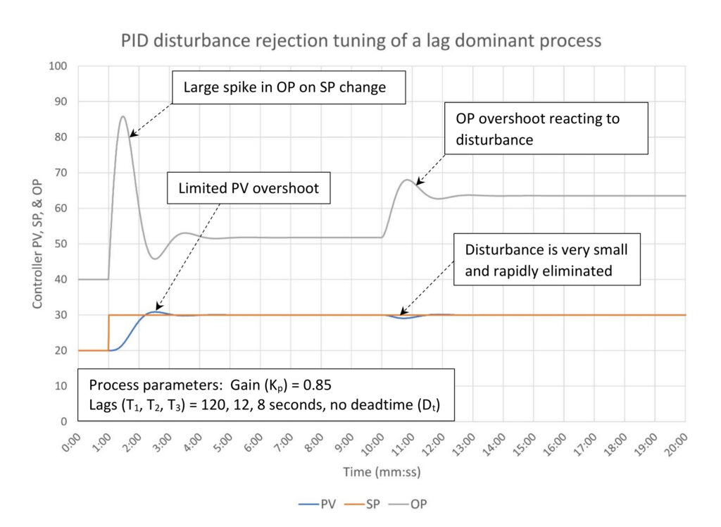
Figure 10: PID controller tuned for disturbance rejection (9.2:1 lag/deadtime ratio). Tuning constants are K = 10.4, Ti = 0.62 minutes/repeat, Td = 0.12 minutes. Integral only on SP change algorithm. Courtesy: Ed Bullerdiek, retired control engineer
Figure 10 is the integral only on SP change algorithm tuned for PID disturbance rejection on our lag dominant process. Compared to figure 1 the controller output (OP) spike after the setpoint change is reduced (the OP doesn’t hit 100%), but it is still too large. On the plus side the process variable overshoot of the setpoint is limited. However, this doesn’t meet our goals.
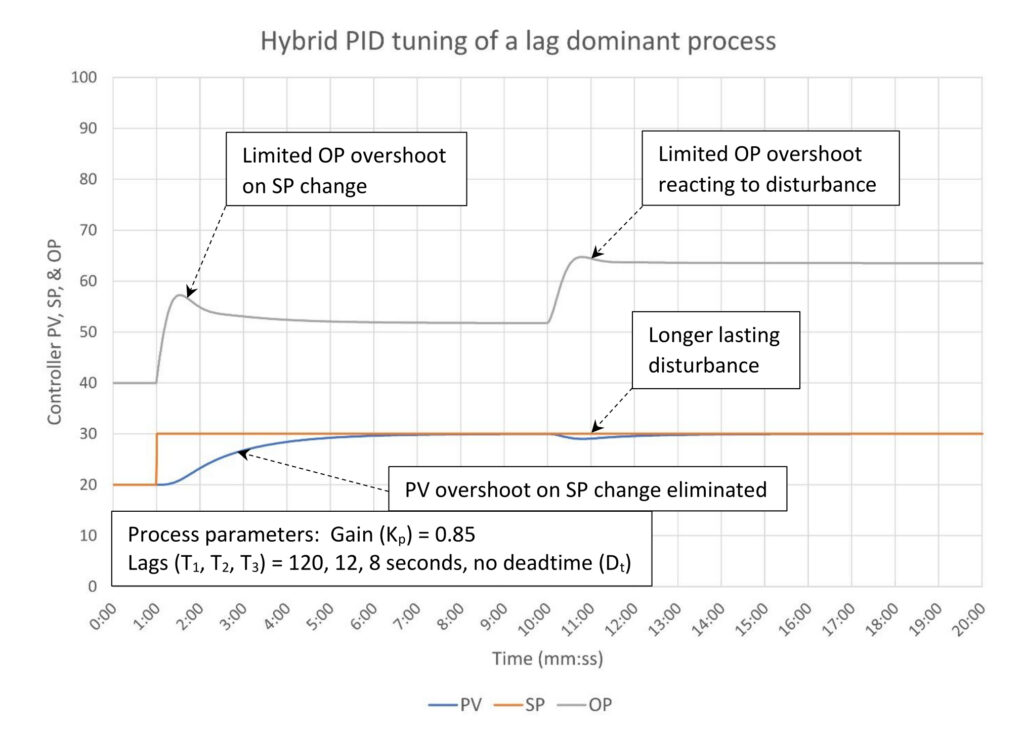
Figure 11: Hybrid PID controller tuning (9.2:1 lag/deadtime ratio). Tuning constants are K = 10.4, Ti = 1.635 minutes/repeat, Td = 0.16 minutes. Integral only on SP change algorithm. Courtesy: Ed Bullerdiek, retired control engineer
Figure 11 is an example of hybrid tuning to achieve competing goals. Controller gain is the primary knob for controlling disturbance rejection, while integral sets the recovery time. In this case, we have retained the high controller gain from disturbance rejection tuning and used the integral time from critically damped tuning to reduce controller output overshoot on the setpoint change (and kept a little derivative to suppress oscillations). The tradeoff we have made is disturbance rejection hardly dropped (90.4% down to 90.2%) while disturbance recovery time changed from 1:25 to 3:58 (the time to return to within 0.1% of setpoint).
The point here is don’t be afraid to mix and match tuning or even work between the tuning windows as necessary to meet your tuning goals.
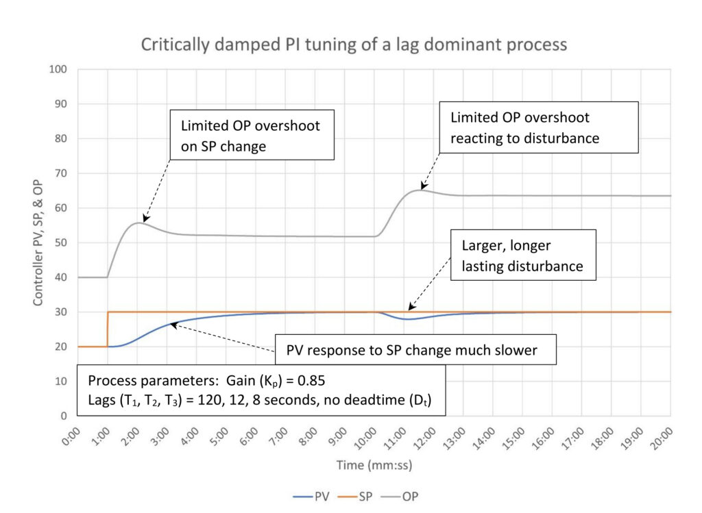
Figure 12: PID controller tuned for critically damped response (9.2:1 lag/deadtime ratio). Tuning constants are K = 4.345, Ti = 1.635 minutes/repeat, Td = 0 minutes. Integral only on SP change algorithm. Courtesy: Ed Bullerdiek, retired control engineer
Comparing figure 12 to figure 2, we can see that the change in algorithm considerably changed the response to the setpoint change. The controller output spike has been largely eliminated, but process variable takes much more time to get to setpoint. However, the controller still retains its “as fast as possible without overshoot” response to a disturbance. For this particular process, the response doesn’t look much different than using a setpoint filter as seen in figure 8.
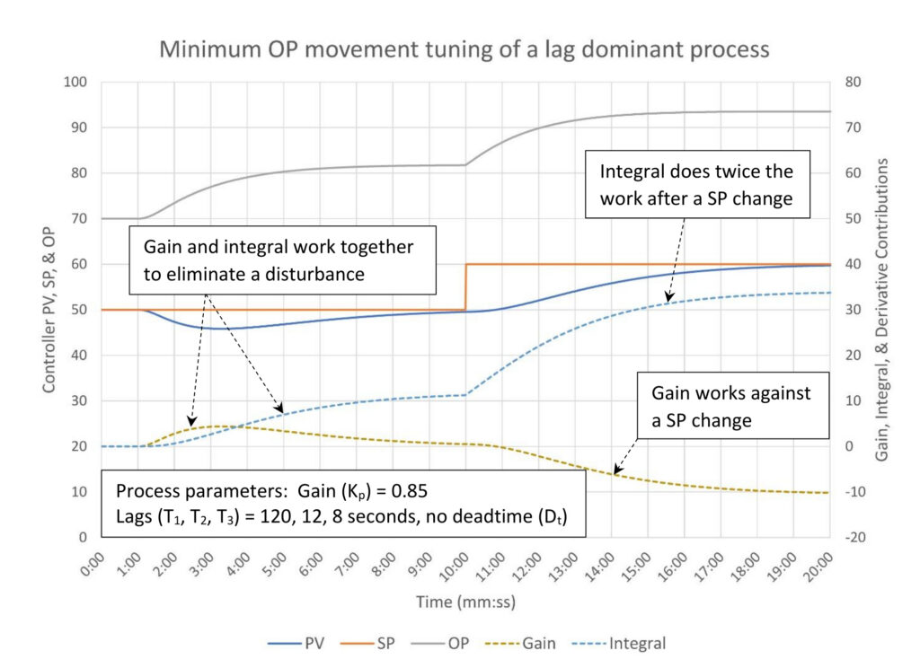
Figure 13: PID controller tuned for minimum output movement response (9.2:1 lag/deadtime ratio). Tuning constants are K = 1.049, Ti = 1.877 minutes/repeat, Td = 0 minutes. Integral only on SP change algorithm. Courtesy: Ed Bullerdiek, retired control engineer
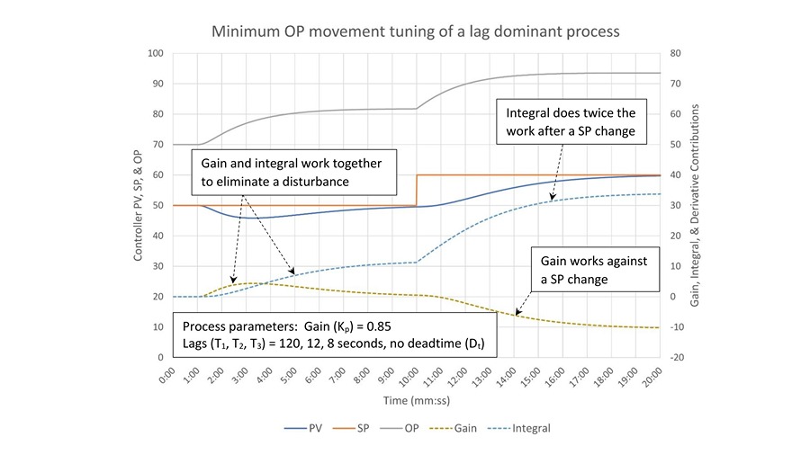
Figure 13 shows a property of the integral only on setpoint change PID algorithm to be aware of. Process variable changes are penalized by the controller regardless of their source. If a disturbance occurs the controller responds exactly like a standard classical PID controller. The controller gain and integral work together to eliminate the disturbance, and when the disturbance is eliminated the gain contribution returns to zero, leaving integral to do all the work.
However, following a setpoint change the controller gain works against the change. The integral action must do twice the work; first to move the process variable to the new setpoint and second to overcome the controller gain’s efforts to return the process variable back to its initial value (PV(t=0)). This slows the response to a setpoint change, perhaps slower than you might have expected.
Advice on using the integral only on setpoint change algorithm
Heuristic tuning and post-tuning performance checks must be done using the induced disturbance test method (see PID spotlight part 17 for how to do an induced disturbance test).
Do not use the integral only on SP change algorithm on a cascade secondary.
Ed Bullerdiek is a retired control engineer with 37 years of process control experience in petroleum refining and oil production. Send comments and questions to [email protected]. Edited by Mark T. Hoske, editor-in-chief, Control Engineering, WTWH Media, [email protected].
Keywords
Proportional-integral-derivative, PID tutorial
Learning objectives
- Understand setpoint ramps, setpoint filters and the integral only on setpoint change PID algorithm.
- Know that these advanced PID features can mitigate excessive controller output movement after a setpoint change, allowing more aggressive controller tuning.
- Understand how controller tuning and the setup of an advanced feature work together to shape controller response.
- Know the basics of how to use and implement these features on different systems.
Consider this
PID controllers are often tuned too slow for proper disturbance control due to excessive controller output movement after a setpoint change. Controller output movement can be managed using one of three advanced controller features available on most systems, which will allow you to unlock your controller’s full potential.
PID series from Ed Bullerdiek, retired control engineer
PID Spotlight, part 1: Three reasons to tune control loops: Safety, profit, energy efficiency
PID spotlight, part 2: Know these 13 terms, interactions
PID spotlight, part 3: How to select one of four process responses
PID spotlight, part 4: How to balance PID control for a self-limiting process
PID spotlight, part 5: What does good and bad controller tuning look like?
PID spotlight, part 6: Deadtime? How to boost controller performance anyway
PID spotlight, part 7: Open-loop tuning of a self-limiting process
PID spotlight, part 8: Closed-loop tuning for self-limiting processes
PID spotlight, part 9: Heuristic tuning for a self-limiting process (part A on heuristic tuning)
PID spotlight, part 10: Heuristic tuning in a self-limiting process
PID spotlight, part 11: How a PID controller works with an integrating process
PID spotlight, part 12: What does good and bad controller tuning look like?
PID spotlight, part 13: Deadtime: what’s the best that I can do?
PID spotlight, part 14: Open loop tuning of an integrating process
PID spotlight, part 15: Open loop tuning of near integrating processes
PID spotlight, part 16: Closed loop tuning of an integrating process
PID spotlight, part 17: Heuristic tuning of an integrating processes
PID spotlight, part 18: Identifying control valve performance problems
PID spotlight, part 19: PID controller tuning mechanics
PID spotlight, part 20: Tuning with bad valves
PID spotlight, part 21: Noise: Can I tune around it?
PID spotlight, part 22: Can I tune a noisy PID controller?
PID spotlight, part 23: Filtering noise for better PID control
PID spotlight: part 24: How do I tune PID controllers during a new unit startup?
PID spotlight, part 25: Navigating PID controller tuning
PID spotlight, part 26: How fast should I tune my PID controller?
PID spotlight, part 27: Navigating PID controller tuning
PID spotlight, part 28: How well will my PID controller work?
More on PID and advanced process control from Control Engineering