How do you make a PID controller ignore small deviations while still responding to large deviations? What is a gap algorithm? Which algorithms work with which systems?
Insights about PID gap control
- Modifying controller gain allows us to shape the PID controller response to meet the process control needs. One form of shaping controller response is gap action; lowering controller gain, and thus the response, when the process variable is close to setpoint and raising it when the process variable is far from setpoint. Gap action can also be achieved by modifying the error calculation outside of the PID controller.
- There are potentially many gap action algorithms. This article describes four; two that modify controller gain and two that modify the error calculation to achieve a gapped controller response.
- The classical and series form of the PID algorithm work well with gain modification gap action algorithms. The parallel algorithm requires separate adjustments to controller gain, integral and derivative; modifying the error calculation is easier. Improper implementation of the notch gap algorithm can lead to “walkaway” and potentially unstable control when the process is noisy. The blended gain notch algorithm works well with noise.
In the next three articles we are going to discuss how to use gap action to improve controller performance. This article will define four gap action algorithms and basic information you will need to know to implement these algorithms. The next two articles will cover:
- How to use gap action to get better disturbance rejection than you would get from fixed proportional-integral-derivative (PID) controller tuning.
- How to use gap action to ignore small deviations while still responding to normal process disturbances. This can help remove unnecessary noise from the process.
What is gap action?
Gap action reduces controller response when the process variable (PV) is close to setpoint (SP), either by changing the controller gain or by modifying how the error is calculated. Which method you choose and how you choose to implement it will depend on the type of PID controller your system uses and whether that PID algorithm uses the “positional” or “velocity” form. Furthermore, the type of problem you are trying to solve will dictate which type of gap action algorithm you should use.
Some systems have gap action built into their PID algorithm. Unfortunately, not all gap action implementations work well. Some have quirks that will perform poorly in certain situations, and some should not be used.
Therefore, your success will depend on understanding the details of your system’s PID algorithm and, if it has built in gap action, understanding the gap algorithm’s details also. Since system documentation very rarely gets deep into the details, this article online walks through how to test your system. A few simple tests will tell you if your PID algorithm is of the “positional” or “velocity” type and whether a supplied gap algorithm will work well. (The oft repeated advice that you should test how your specific system works is especially important when it comes to advanced features. There are no standards and, based on my experience, sometimes insufficient regard for how these features will work in practice.)
Gap action using controller gain
If your control system uses the classical or series form of the PID algorithm gap action can be implemented by changing the controller gain. These algorithms multiply the integral and derivative action by the controller gain, thus maintaining the ratio between the three parts of the controller. The parallel algorithm requires changing gain, integral and derivative proportionally to provide gap action; it may be easier to modify the error calculation instead.
Two forms of controller gain gap action available on commercial systems include:
- Notch gain: Reduces controller gain when the PV is close to the SP. The controller gain inside the notch may go as low as zero. This should only be used with the velocity form of the PID controller.
- V-notch gain: The controller gain increases linearly with the distance of the PV from the SP (the error). The controller gain at SP may be zero. This will work with either PID form, but the behavior will be different.
Of course if your system allows external programming to change the controller gain you can perform any kind of gain manipulation you want. However, if your system uses the positional PID form the gain calculation must be continuous. Discontinuities (the gain makes sudden jumps) will cause the controller output to make sudden jumps. The velocity form tolerates discontinuities, but there are tradeoffs here also.
Gap action using controller error
If your system uses the parallel PID algorithm or does not permit a program to change the controller gain the other way to shape controller response is to change how the error is calculated. Here are two gap algorithms that have been used:
- Error squared: The error presented to the PID controller increases as the square of the distance of the PV from the SP.
- Floating SP gap: The SP is matched to the PV within the gap, resulting in an error of zero being presented to the PID controller. If necessary a rate limit may be applied to the SP within the gap to provide positive control if the PV is moving too quickly through the gap.
These two work with any form of the PID algorithm because the error is programmed outside the PID function. Some systems have a PID on error function that expects an error to be fed to the function (and no input for the SP). If your system does not offer this a regular PID controller can be used by connecting the error calculation to the PV input and locking the SP at zero. Depending on system design a custom operator interface may be required.
Notch gap gain
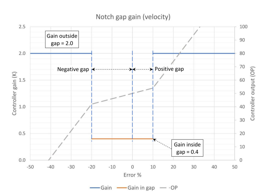
Figure 1 is a visual depiction of a notch gap gain application. There are three configuration parameters:
• Positive gap; the gap above the setpoint
• Negative gap; the gap below the setpoint
• Gap gain multiplier (range 0-1); how much to reduce the controller gain inside the gap.
In Figure 1 the configuration is positive gap is 10%, negative gap is 20%, the controller gain is 2.0 and the gap gain multiplier is 0.2, which results in a controller gain inside the gap of 0.4 (2.0 * 0.2). Separate gaps allow (for example) a narrow gap, or no gap, on the side of the setpoint where a higher controller gain is required. This could be used for constraint control, where being on the safe side of the constraint doesn’t require aggressive control.
The controller output (OP) is included in Figure 1 to check whether the proposed scheme will fully open/close the output assuming the setpoint starts at 50%. This is calculated for a gain only controller. This is not necessary for a self-limiting process, but it is very useful when planning gap action for integrating processes. Figure 1 confirms that for this gap control setup the OP will fully close and open within 50% of setpoint, which makes me feel comfortable that this controller would keep a level from running dry or overfilling.
V-notch gap gain
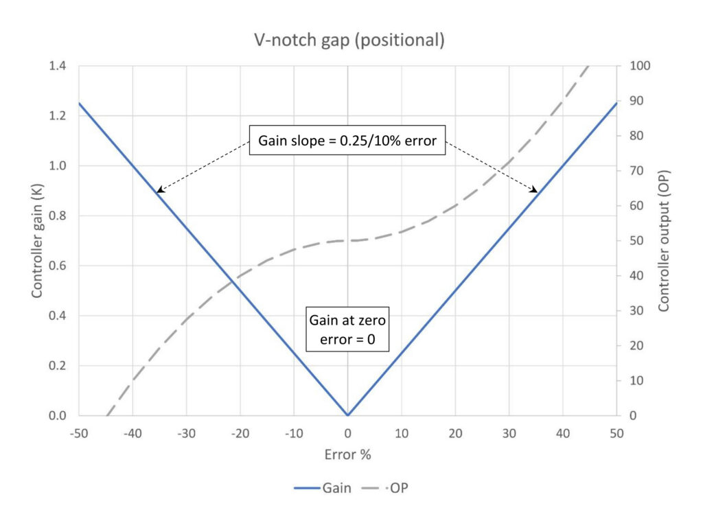
A V-notch gap is shown in Figure 2 for a positional PID algorithm. The gap setup, however it is defined, requires a base gain when the error is zero and a slope for the gain on either side of zero. When used with the positional PID algorithm, this produces an S-shaped controller output. The controller will be less sensitive to small changes near the setpoint and will respond strongly to large errors. This does not provide the asymmetry needed for (for example) one-sided constraint control. However, you could write a custom version of the V-notch gap action with different slopes on either side of zero and/or a flat spot at the bottom. The key point here is for positional PID algorithms you cannot have a discontinuity in the controller gain.
Error squared gap
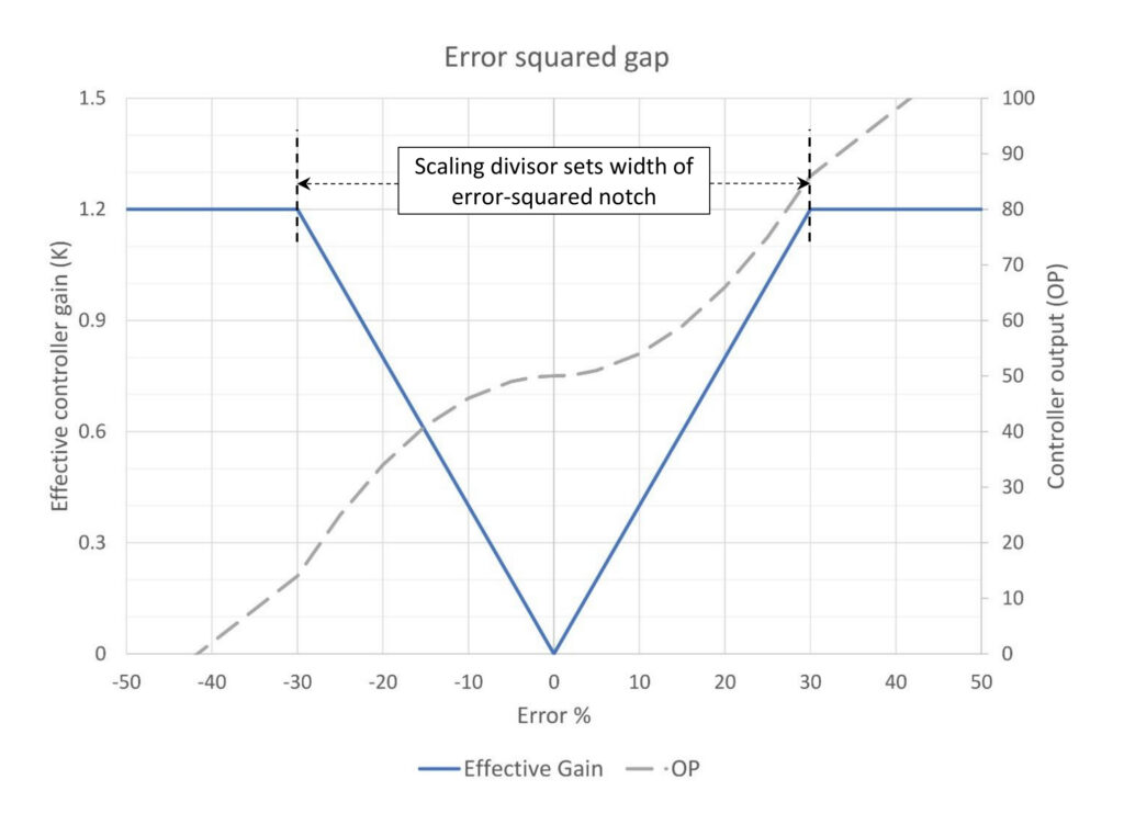
Figure 3 shows the effective controller gain profile for error squared gap and the controller output shape for gain only control. Error squared is functionally identical to V-notch gain but has the advantage that it will work with the parallel PID algorithm or any system that does not permit changing controller gain. The width of the notch is set by the scaling divisor; when the error exceeds the scaling divisor the PID controller is fed the error instead of the square of the error. This prevents excessive controller action on large errors.
The error squared algorithm does not permit a non-zero effective controller gain when the error is zero nor does it permit nonsymmetrical controller response to error. Therefore it will not be appropriate for constraint control.
Floating setpoint gap
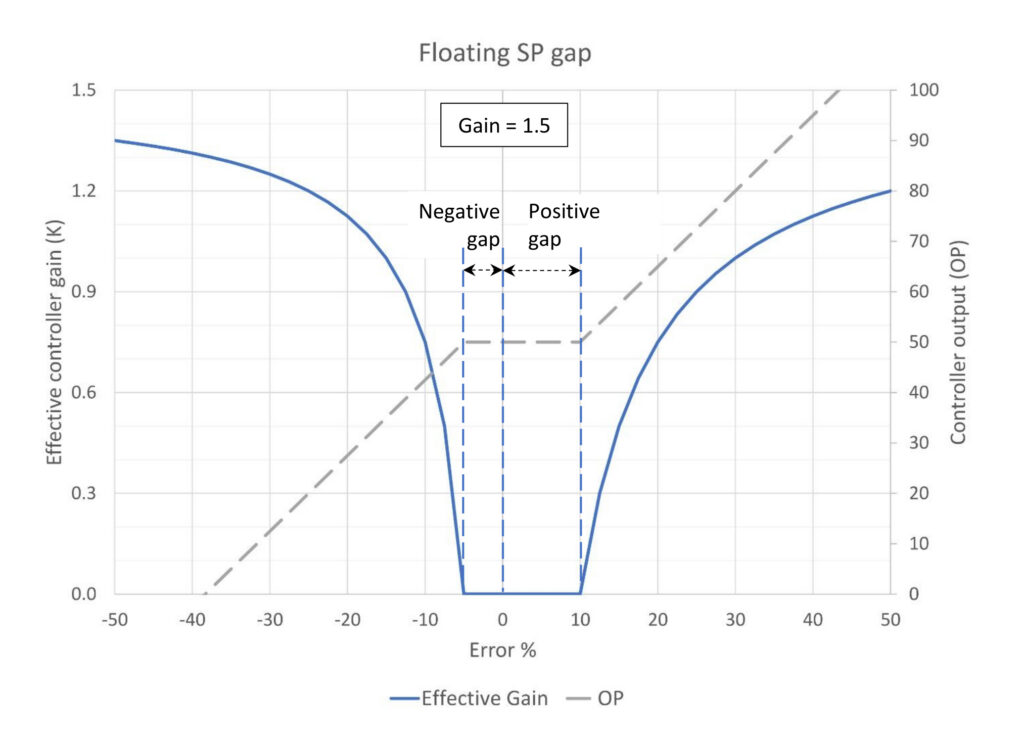
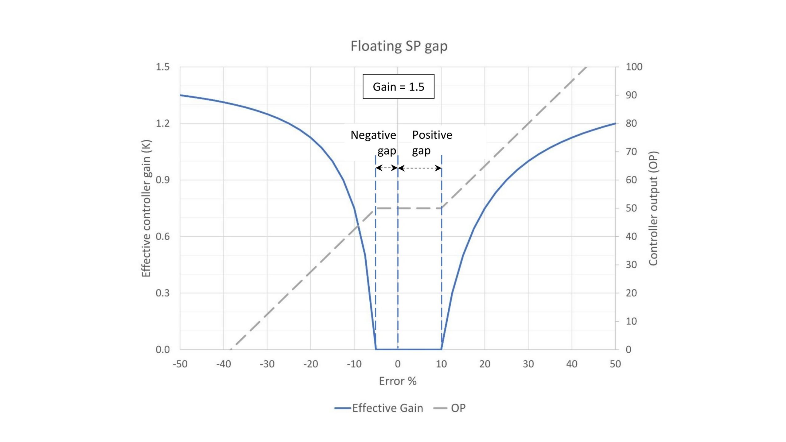
The floating setpoint gap algorithm forces the SP to follow the PV inside the gap, thus calculating zero error. The controller output (OP) will remain constant as long as the PV is inside the gap. When the PV gets outside the gap the edge of the gap is used in the error calculation. This results in the OP profile seen in Figure 4, where the OP starts moving smoothly at both ends of the gap without objectionable jumps. The high and low gaps are configured separately, permitting an offset setup useful for constraint control. In Figure 4 the high gap is 10%, the low gap 5% and the controller gain is 1.5.
How fast the SP is allowed to follow the PV within the gap can be rate limited. This is not needed for self-limiting processes, however it can be used to prevent ping-ponging in integrating processes. (Integrating processes are notorious for bouncing between the high and low limits of a gap controller, confounding efforts at surge control. Providing a little restraint on the SP speed through the gap will provide some positive control of the PV, which will suppress if not outright stop the ping-pong effect.)
Identifying your PID algorithm
Identifying the PID algorithm used by your system shouldn’t be difficult, but then again, we’ve all spent way too much time digging through system documentation looking for some magic nugget of information. In the unfortunate case where the system documentation is hopelessly opaque or simply doesn’t exist (which might be a blessing), a couple of methods can help.
If the control system either has an “integral only” function, or the PID block offers a configuration option titled “integral only” it is safe to assume that the normal PID algorithm is classical. In the parallel PID algorithm the integral action is completely independent from controller gain, which means there is no need for a special function or configuration option to permit “integral only” control.
This brings us to the second option to determine the PID algorithm – testing. If you have access to a system emulator, a test system or have a safe space on your system to set up a test PID controller, you can configure a PID function with zero controller gain and some integral action. Then introduce some error (PV not equal to the SP) and, if your system uses the parallel algorithm the controller output will move. If not, the system most likely uses the classical algorithm.
Is my PID controller positional or velocity?
System documentation does not discuss this because (I’m speculating) it touches on the proprietary details of the vendor’s PID algorithm. Nor does it receive much attention in textbooks. The short answer is the positional form calculates the controller output using the PID equation as written (from PID spotlight part 2):
OP = K *(Error + 1/Ti*∫Error + Td*d(PV)/dt) + OP(t=0)
Digital control systems work on fixed time intervals, which for programming purposes means the positional form of the classical PID equation is this difference equation:
OP = K *(Error + 1/Ti*ΣError0→n + Td*ΔPV) + OP(n=0)
Where Δ is shorthand for the difference between execution intervals (PV(n) – PV(n-1)).
This omits the details necessary to keep track of the execution interval in the interest of clarity.
The problem with the positional form is if you change the controller gain while the controller is running, there will be an immediate change in controller output. This will bounce your process.
The solution is to calculate the change in controller output each execution interval and add it to the previous output calculation. This is the velocity form of the PID equation.
OP = K *(ΔError + 1/Ti*Error + Td*ΔΔPV) + OP(n-1)
This glosses over a bunch of implementation details, and there are many possible ways to implement this in code. The key things to note here is that the “integral” term no longer includes the summation of error from when the controller was first turned on, it’s no longer an integrator, and the output bias term (OP(n=0)) has been replaced with the controller output from the prior execution. This untethers the PID execution from the initial position of the controller when it was first placed in automatic, plus any accumulated history is now included in the controller output from the previous cycle. (For the calculus nerds among us this is the first derivative of the positional form of the PID equation.)
The net impact of this is we can now change the controller gain on the fly without the controller output jumping. This tells us how we can check to see if the PID controller form is positional or velocity:
- Set up a gain only controller with a fixed PV.
- Set the controller SP at a different value than the PV. The controller OP will settle at a new position.
- Once the OP has stopped moving change the controller gain.
- If the OP moves the controller form is positional. If it stays the same it is velocity.
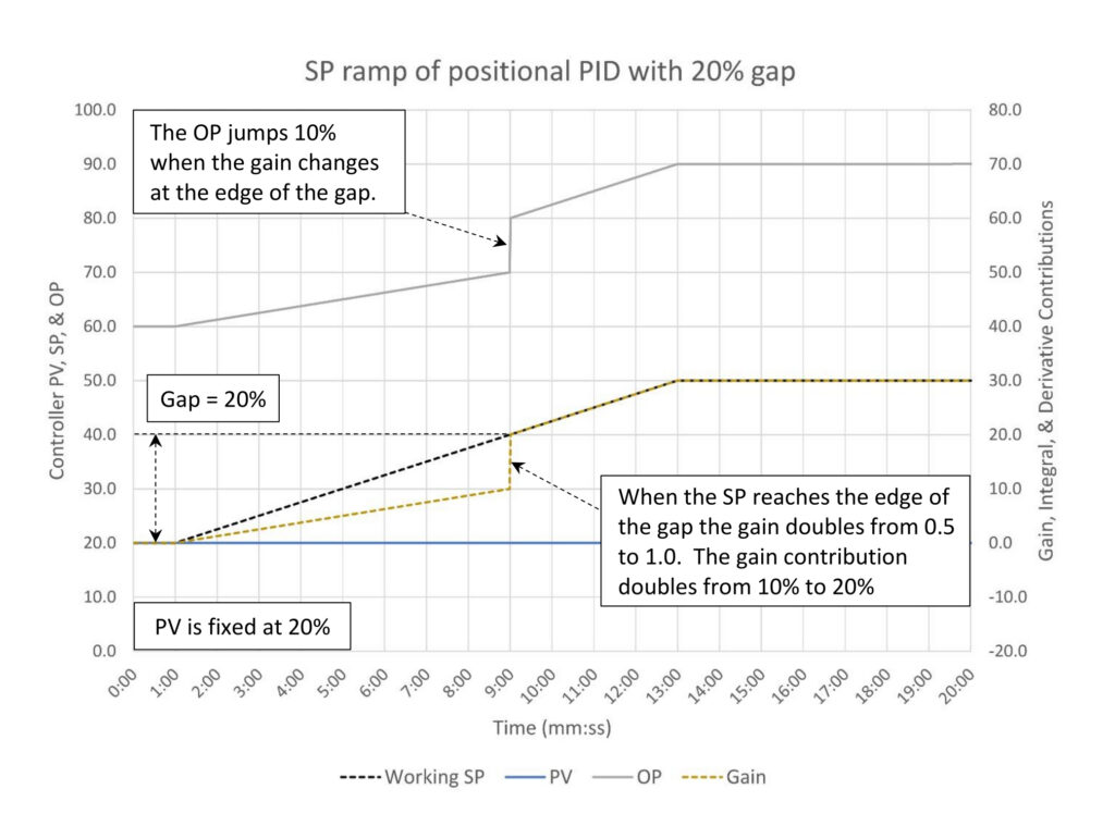
Figure 5 illustrates the problem that occurs when the positional form of the PID algorithm encounters a discontinuous change in controller gain. When the error crosses the 20% edge of the gap the controller gain changes from 0.5 to 1.0, which causes the gain contribution to jump with the change in gain. This, of course, results in a 10% jump in the controller output. We can use gain scheduling with a positional algorithm, but we must make sure that the gain schedule is continuous and reasonable. It would be best to build a controller output position versus gain chart similar to Figure 2. And for our immediate discussion the notch gap feature should not be used even if it is offered.
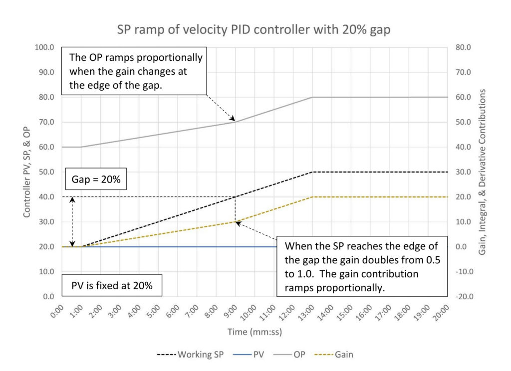
Figure 6 provides a much more encouraging picture of how the velocity form of the PID algorithm responds to a discontinuous change in controller gain. The sudden change in controller gain when the error crosses the gap threshold at 20% doesn’t cause a controller output jump, but instead simply changes the ramp rate proportionally to the SP ramp rate. This not only makes it easier to implement notch gaps but any custom form of gain scheduling that might be required for (for example) split range valves.
Implementation details for notch gap gain
Once you have verified that the PID controller uses the velocity form, you must still pay attention to the implementation of the notch gap gain algorithm. The temptation will be to use the gain at the current PV, and some commercial applications do this. Figure 7 illustrates the problem with this approach; if the process variable steps over a gap limit multiple times, the controller output can walk away. This is not a problem when the PV moves are contained inside the gap, nor when the PV moves occur fully outside the gap. Inside the gap (0-5 minutes) the OP step size is 1.25% both up and down. Outside the gap (5-10 minutes) the OP step size is 5% both up and down.
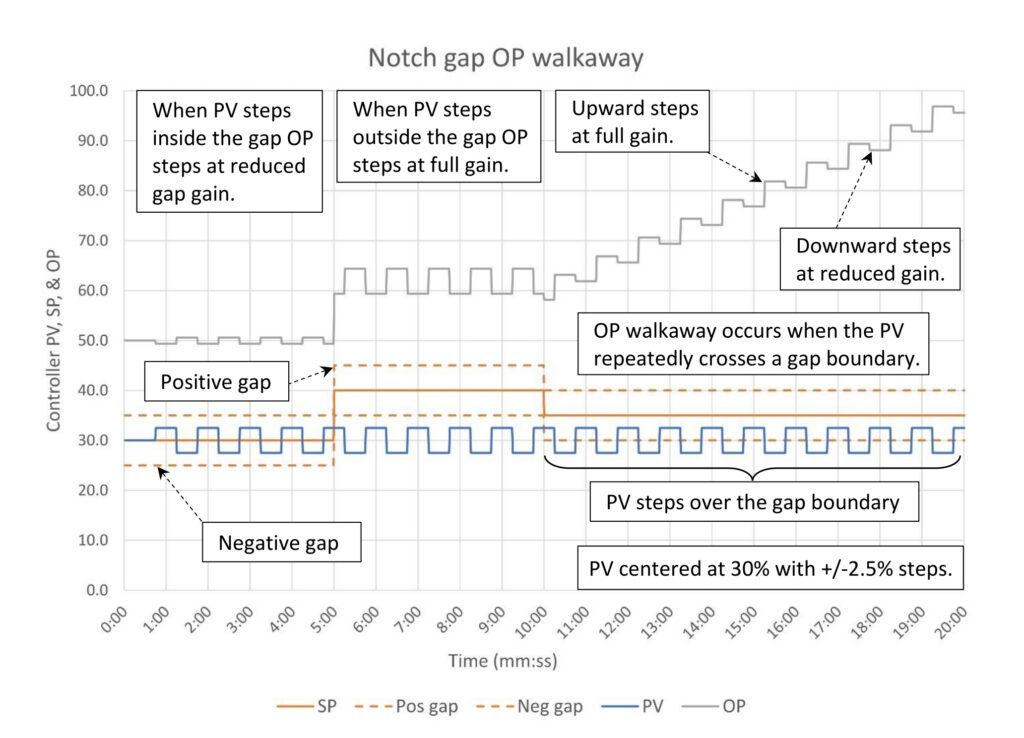
However, when the PV steps over the gap boundary (after 10 minutes), the upward OP step size is calculated using the full controller gain of 1.0, and the step size is 5%. The downward OP step size is calculated using the gap controller gain of 0.25, resulting in a step size of 1.25%. This mismatch in upward and downward step size results in walkaway. If this happens once or twice it might not be a huge issue, but if the process has noise and some deadtime the OP could walk enough to cause oscillations and instability.
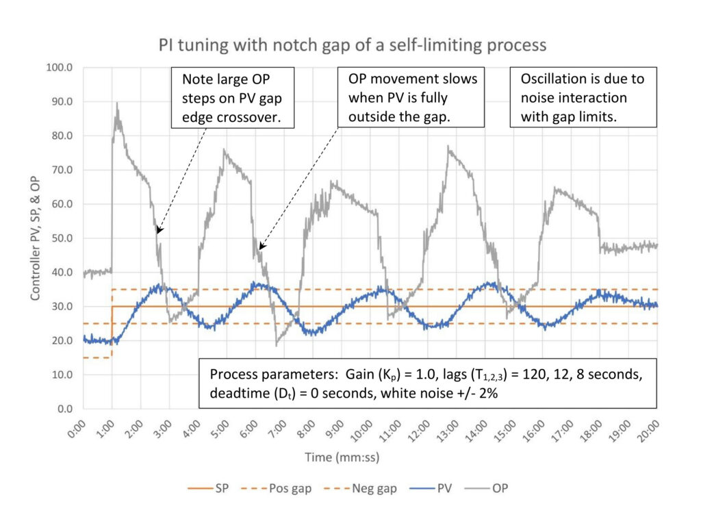
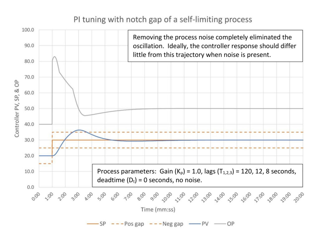
In Figure 8 we can see that a relatively small amount of noise can cause oscillation even where we shouldn’t expect any. The controller is tuned for slightly faster than critically damped response outside the gap and for about minimum OP movement inside the gap. This will result in some PV overshoot on a setpoint change, but we should not expect to see more than the tiniest oscillation (see Figure 9).
But the addition of just +/-2% white noise causes rapid OP walkaway whenever the process variable meets a gap limit. The mechanism is as seen in Figure 7, when the PV steps over the gap limit repeatedly the OP walks too far and causes overshoot in the opposite direction. If it is bad enough the process can go unstable. (I was very puzzled when I first ran across what appears to be bizarre behavior. This one took some time to run down, so it’s worth covering in detail.)
We are going to explore using very aggressive tuning combined with gap action to provide better disturbance rejection while maintaining stability in situations where disturbance rejection is very sensitive to controller gain. If a little bit of noise can effectively make this impossible this removes a potentially useful tool from our toolbox. It is incumbent upon us to find a better way to do gap control.
There are three ways to mitigate the OP walkaway problem; when stepping across the gap boundary always use the controller gain, always use the gap gain or calculate a blended controller gain. The first two may still have some tendency for the OP to walk depending on the pattern of the gap crossings. Calculating a blended gain is more difficult but is guaranteed to avoid OP walkaway.
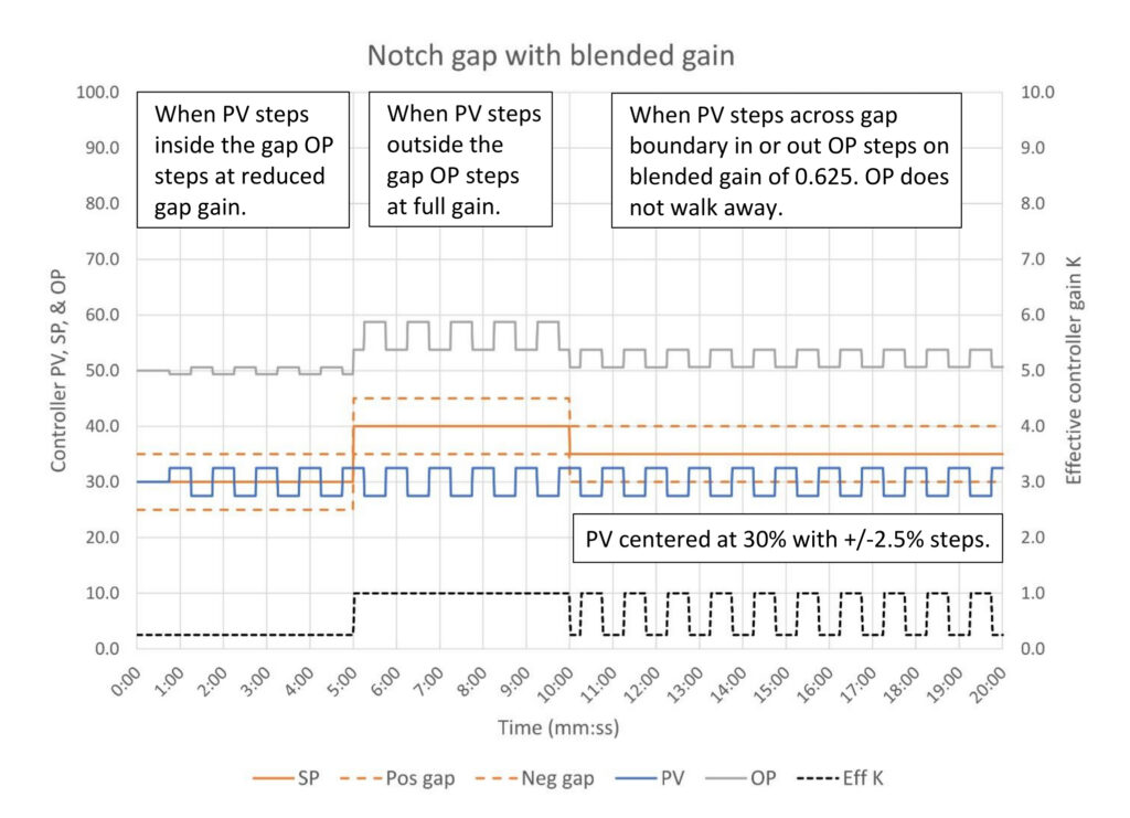
Figure 10 is a repeat of the notch gap test run in Figure 7, but the notch gap algorithm calculates a blended gain whenever the PV crosses the gap boundary. Unlike Figure 7 the controller output does not walk when the PV repeatedly crosses the same boundary because the blended gain is always the same regardless of the crossing direction. In this case the blended gain is 0.625, calculated based on the PV swapping between 2.5% above and below the gap boundary, the controller gain equal to 1.0, and the gap gain multiplier being 0.25.
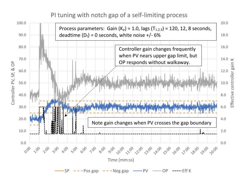
Figure 11 gives us proof of concept for using blended gain in the notch gap calculations. It worked so well with the tuning used in Figure 8 that I ventured to see how far the tuning could be pushed. This ended at PI disturbance rejection tuning, with controller gain raised 50% (6.0 versus 4.0) and integral sped up (more than halved at 0.7 versus 1.5 minutes/repeat). This much more aggressive tuning still functions despite tripling the noise (+/- 6% versus 2%).
This tuning is not recommended; it’s on the very edge of stability. Adding a 6 second filter to knock down the noise pushes this process into instability. This is not a surprise. The process has a lag/deadtime ratio of 9.2:1; adding the 6 second filter drops the lag/deadtime ratio to 6.8:1. This points up again the problem with using filtering for noise suppression. Adding the filter dropped the lag/deadtime ratio 26%, which significantly limits the controller gain which, if you are really trying to push performance may cause a problem.
Note that when the noisy PV slightly crosses a gap boundary that the effective controller gain trend does spike up a little bit. These little spikes have the effect of herding the PV inside the gap. This is a tool we may be able to use to reduce filtering to preserve controller effectiveness while still reducing valve movement while the PV is close to setpoint.
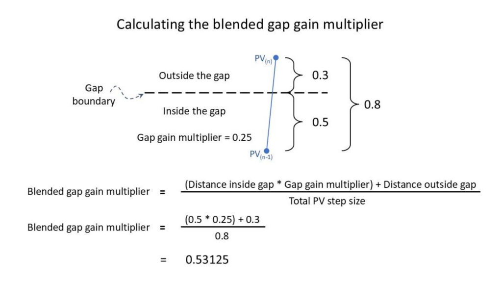
Figure 12 covers the basics of calculating the blended gain gap multiplier. While the details will be different based on the system, the core is to calculate a controller gain that is somewhere between the full controller gain and the controller gain inside the gap when the PV steps over a gap boundary. In this system the gap gain multiplier is a number between zero and one, which is then multiplied by the base controller gain to get the gain inside the gap. The blended gain multiplier is going to be somewhere between the programmed gap gain multiplier and one. In Figure 11 we can see how the effective gain (Eff K) plot jumps whenever the PV steps over a gap boundary but is always between 6.0 (the controller gain) and 1.5 (the controller gain times the gap gain multiplier: 6.0 * 0.25).
In Figure 12 the PV stepped from 0.5 below the gap boundary (PV(n-1)) to 0.3 above the gap boundary (PV(n)). The blended gap gain multiplier will equal the weighted average of the distance inside and outside the gap. Note that the direction doesn’t matter. If the PV jumps back to 0.5 inside the gap, during the next execution the blended gap gain multiplier will be the same, as it needs to be to prevent walkaway.
Finally, if the PV jumps completely over the gap (PV(n-1) is below the low gap limit and PV(n) is above the high gap limit) then the calculation must be weighted to include the total distance the PV traveled outside the gap and the distance across the gap. This will prevent anomalous behavior should the PV step from inside the gap to outside, then step across the gap, and then step back inside the gap. The goal of the calculations is to have fully repeatable behavior regardless of direction or step size.
Implementation details for V-notch gap gain
Changing controller gain on a positional PID controller is repeatable, which means we don’t have to worry about how the controller will respond to noise. The programming is as simple as setting a baseline controller gain and a ramp on either side or setpoint. The commercial versions set the ramp on either side of the setpoint the same, however, a programmed solution could be set up with different ramps on either side of the setpoint, or none at all on one side if enhanced constraint control is the goal. Custom solutions should be modeled to verify they meet the needs of the process.
Implementation details for error squared gap
The idea behind the error squared PV gap algorithm is to modify the PID controller’s behavior by feeding it a calculated non-linear PV error signal. This is used on systems that do not permit changing the controller gain while the PID controller is running or uses the parallel PID algorithm.
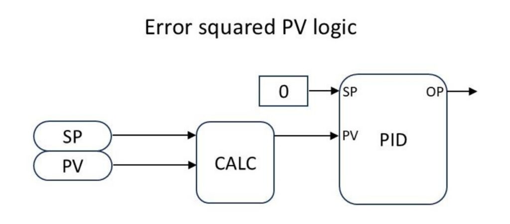
Figure 13 is simplified sample logic to illustrate the calculation process and to highlight one of the potential problems with feeding the PID block with a calculated error signal. If your system’s graphic shapes, faceplates and detail displays access the controller PV, SP and OP directly from the PID function block this logic will require custom versions of all three. If your system provides a separate controller interface block (sometimes called a manual/auto station), this approach has less overhead.
The setpoint to the PID controller block must be zero. Lock this to prevent accidental changes (and prevent a midnight callout or two.)
The basic error squared on PV calculation is:
Error squared = Error * ABS(Error) / Scaling divisor
Multiplying the error times the absolute value of the error preserves the direction of the error (plus or minus) so the PID controller will respond in the right direction. The scaling divisor sets how rapidly the error squared signal increases. A larger divisor reduces the aggressiveness of the calculation.
If necessary the aggressiveness of the calculation can be limited by substituting the true error whenever the absolute value of the true error is greater than the scaling divisor (see Figure 3):
PV to PID = If(ABS(Error) > Scaling divisor, Error, Error squared)
Implementation details for floating setpoint gap
The floating setpoint gap works by matching the setpoint to the process variable within the gap and calculating an error equal to the distance of the process variable from the edge of the gap when the process variable exceeds the gap limits. This provides the smooth controller response seen in Figure 4.
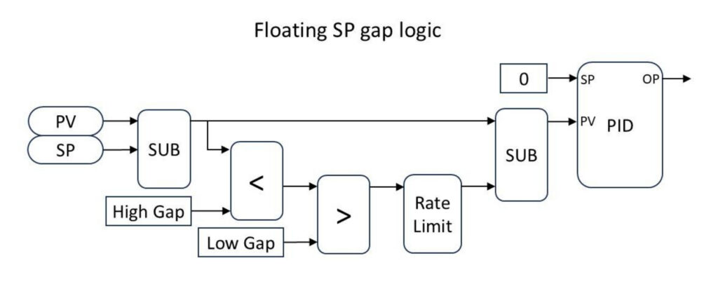
Figure 14 is simplified function block logic that performs the gap logic by first calculating a raw error, then clamping the error at the gap limits and subtracting that error from the raw error. The end result is zero if the error is inside the gap limits and the difference between the raw error and the clamped error if the error is outside the gap limits. The rate limit block will provide positive control if the PV is moving through the gap too fast. As mentioned above, this isn’t useful for self-limiting processes, but can mitigate or eliminate ping-ponging in integrating processes.
A final note about gap control
Gap control is one of several options to shape controller response to master problems a pure linear PID controller cannot handle well. Gap control gives you more options, but increased complexity comes with these additional options. In refining gap action is used infrequently, in part because of the additional complexity and also because the effort isn’t often justified. Getting a controller set up properly will include some combination of modeling and revisiting the tuning to verify it is working as intended. This limits the effort to high value controllers.
That said, gap action is used often enough that vendors have supplied gap action options in their systems. Unfortunately, as noted above, sometimes these options do not work as we would like them to. This turns our decision on whether to use the provided gap action option into a research project. While this is not terribly difficult it requires resources and time, something that is often in short supply.
Ed Bullerdiek is a retired control engineer with 37 years of process control experience in petroleum refining and oil production. Send comments and questions to [email protected]. Edited by Mark T. Hoske, editor-in-chief, Control Engineering, WTWH Media, [email protected].
Keywords
Proportional-integral-derivative, PID tutorial
Learning objectives
- Understand PID controller gap action and know four gap algorithms.
- Know how to identify the system’s PID algorithm and which gap action algorithm works best with each. Also Know the difference between the positional and velocity PID algorithm variants and which gap action algorithm can be used with each.
- Know the implementation details for four gap action algorithms.
Consider this
Do you understand why notch gap algorithm implementation details are important and how to test for faulty applications?
Extra online
Five more pages of explanation and examples appear with this article online with 10 more graphics, System documentation very rarely gets deep into the details; this online version walks you through how to test your system.
PID series from Ed Bullerdiek, retired control engineer
PID Spotlight, part 1: Three reasons to tune control loops: Safety, profit, energy efficiency
PID spotlight, part 2: Know these 13 terms, interactions
PID spotlight, part 3: How to select one of four process responses
PID spotlight, part 4: How to balance PID control for a self-limiting process
PID spotlight, part 5: What does good and bad controller tuning look like?
PID spotlight, part 6: Deadtime? How to boost controller performance anyway
PID spotlight, part 7: Open-loop tuning of a self-limiting process
PID spotlight, part 8: Closed-loop tuning for self-limiting processes
PID spotlight, part 9: Heuristic tuning for a self-limiting process (part A on heuristic tuning)
PID spotlight, part 10: Heuristic tuning in a self-limiting process
PID spotlight, part 11: How a PID controller works with an integrating process
PID spotlight, part 12: What does good and bad controller tuning look like?
PID spotlight, part 13: Deadtime: what’s the best that I can do?
PID spotlight, part 14: Open loop tuning of an integrating process
PID spotlight, part 15: Open loop tuning of near integrating processes
PID spotlight, part 16: Closed loop tuning of an integrating process
PID spotlight, part 17: Heuristic tuning of an integrating processes
PID spotlight, part 18: Identifying control valve performance problems
PID spotlight, part 19: PID controller tuning mechanics
PID spotlight, part 20: Tuning with bad valves
PID spotlight, part 21: Noise: Can I tune around it?
PID spotlight, part 22: Can I tune a noisy PID controller?
PID spotlight, part 23: Filtering noise for better PID control
PID spotlight: part 24: How do I tune PID controllers during a new unit startup?
PID spotlight, part 25: Navigating PID controller tuning
PID spotlight, part 26: How fast should I tune my PID controller?
PID spotlight, part 27: Navigating PID controller tuning
PID spotlight, part 28: How well will my PID controller work?
PID spotlight, part 29: How to shape PID controller response – part 1
PID spotlight, part 30: How to shape PID controller response – integrating processes
More on PID and advanced process control from Control Engineering