PID-correction-based control system implementation

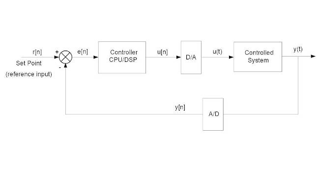
While dealing with the control system synthesis in s-domain is completely logical as the controlled systems operate continuously (in time), the control system implementation is however another matter. Today, almost all control systems are implemented as digital systems, based either on the microprocessors (microcontrollers), or on the digital signal processors as shown in Figure 1.

Figure 1, COVER: Block diagram shows a digital closed-loop control system. Courtesy: Peter Galan, retired control software engineer

PID for a discrete-time control system

The analog PID controller, which is still considered as the most powerful (Figure 2), can be modified for implementation as a discrete-time control system, as it is not difficult to rewrite its differential Equation 1 into its difference form (Equation 2)

where u[n] is the actuating value at the present time n, e[n] is the regulation error at the time n and e [n-1] is the regulation error at the previous sample time, n-1. T is the time period of the sampling. The same time period, T, is used for the processing, that is, for the u[n] calculation.

For the practical applications Equation 2 requires certain modifications, beginning with the integration member. The integration member adds each value of the regulation error to a sum and then multiplies this sum by the time constant and by the integral constant. If the value of the time or integral constant suddenly changes (which can happen, especially during the tuning process), the actuating value will change abruptly and cause problems. A better approach is to multiply the regulation error by those two constants first and only then to accumulate their product. Another improvement can be achieved by using the trapezoidal approximation of integration instead of the rectangular one.

How to reduce noise

The derivative member of Equation 2 is a second source of problems. In its simple form, this member tends to be rather noisy. To reduce noise, you can use more than two (for example four) consecutive samples of the regulation error. The result is as if the difference of the regulation error went through a tiny (4-tap) finite impulse response (FIR) filter.

The modified PID formula then appears as the following Equation 3

The difference equation above can be implemented in any programming language and for any microprocessor/microcontroller.

Figure 2: PID controller calculates an actuating value from proportional, integral, and derivative components. Courtesy: Peter Galan, retired control software engineer

Interrupt service routine

Still, there is one open question with regard to the sampling/processing period, T. What is the correct control process period (frequency), and what does it depend on? The control frequency depends only on the time constant of the closed-loop transfer function. Remember, this time constant can be an order shorter than the time constant of a controlled system itself. Optimally, you should run the control procedure around 5 to 10 times more often than what is the value of the closed loop time constant, τ. Immediately, before your control procedure starts to run, you should have the latest samples of r[n] and y[n] ready (see Figure 1).

The best arrangement is if the control procedure is called as an interrupt service routine (ISR) triggered be the A/D converter providing the y[n] value. Result of the control procedure calculation, the actuating variable u[n], should be sent out to the D/A converter as soon as possible. Otherwise, the transfer function of the controlled system will be affected by transportation delays, which could destroy (make it unstable) the control system.

To avoid the noise, which can always penetrate into the control system from the outside (for example as the “board” noise caused by electronic parts, mainly switching power supplies), all the measured variables – signals like y(t), have to be thoroughly filtered. They should “go through” a proper anti-aliasing filter, with the cut-off frequency well below one half of the sampling frequency, 1/T, If, for some reason, they cannot be filtered by proper analog filters, they should be at least over sampled and filtered digitally.

More on the PID control transfer function

Equation 3 is not the only way for the discrete implementation of a PID controller. Another possibility is the transformation of a PID control transfer function from its s-domain (Equation 4) into z-domain. In practice, there are two ways of such a transformation. Both are derived from a different approximation of a discrete time integration. The most common approximations of the discrete time integration is a rectangular (Equation 5) and a trapezoidal (Equation 6) approximation.

If you express  in the z-domain, for the rectangular approximation you will get

And this is what you get for the trapezoidal approximation:

Equation 7 and 8 correspond to the integration term, which in the s-domain is expressed as 1/s. So, if you take the reciprocal expression of the right side of the Equation 7 (expressing s) and substitute with it each s operator in the Equation 4, you will get the following transfer function of the PID compensation (in the z-domain):

Similarly, if you take the reciprocal expression of the right side of the Equation 8 and substitute with it each s operator in the Equation 4, you will get the following transfer function of the PID compensation (in the z-domain):

Control system modelling in z-domain

Equation 9/10 can be suitable for modeling of the control systems in z-domain, for example in Matlab, but cannot be directly implemented by any controller. However, after applying an inverse z-transform to Equation 9, you will get the following equation

and an inverse z-transform of Equation 10:

Equation 11 and Equation 12 are perfectly suitable for implementation on any microprocessor (microcontroller) or a digital signal processor. If you keep K₁, K₂ and K₃ as the pre-calculated constants (instead of variables), the entire control procedure will require three multiplications, four additions and remembering four previously calculated variables – two regulation errors, e[n — 1] and e[n — 2], and two actuating variables, u[n — 1] and u[n — 2] (only for Equation 12). The e[n] calculation requires one subtraction.

Infinite impulse response filters

You can go even further in the optimization of your control procedure. The digital signal processing industry has very popular recursive filters, so-called infinite impulse response (IIR) filters. Usually, they are implemented as cascaded, second-order filters. One such second order filter, often called as “biquad” (biquadratic), converted to its canonical form, which is called Cascade Form II, is shown in Figure 3.

Figure 3: Second-order canonical IIR filter section serves as a PID controller. Courtesy: Peter Galan, retired control software engineer

Implementation of such a biquad requires less memory space – instead of four variables – delayed terms e[n — 1], e[n — 2], u[n — 1] and u[n — 2], it is only necessary to remember two state variables, and d[n — 1], d[n — 2]. The canonical IIR filter section is best described by the following two difference equations

You have some, though limited choice for the A₁ and A₂ values selection. However, two rules have to be obeyed: the sum of A₁ and A₂ values has to be always 1.0, and no value can be greater than 1.0. So, you can use as the A₁ and A₂ coefficient, for example, values like 1.0 and 0, or 0.5 and 0.5, or 0 and 1.0, or anything in between.

The last combination will yield the identical response as Equation 12 The lower the A₂ value, the faster is the control system response. This can simplify the tuning process, as instead of frequently modifying the K_I value (which requires re-calculation of the K_P and K_D values if you want to have them optimal, that is, cancelling the controlled system poles) you can set the K_I constant (and the K_P and K_D values) once to some reasonable value, for example K_I to the  value (where τ₁ and τ₂ are the primary time constants of the controlled system) and make the final tuning by the adjustment of the A₁ and A₂ values.

Not every PID implementation is satisfactory

While it is always nice to have a choice when any algorithmic problem has to be implemented, not every implementation provides satisfactory results. The same applies to the described PID control procedures. All three procedures work nicely on paper, but when implemented, problems will occur.

While the first, Equation 3, implementation requires more mathematical operations (multiplication, additions) and remembering more previous results than the remaining two, it provides very smooth results. The behavior of Equation 11 is similar.

However, implementation of Equation 12 will fail to deliver satisfactory results, as it runs on the border of stability, and its output will permanently oscillate. The Equation 13/14 implementation will work properly, but the A₁ coefficient must be kept > 0 because otherwise it will behave exactly like the Equation 12 implementation and produce permanent oscillations.

Peter Galan is a retired control software engineer; Edited by Mark T. Hoske, content manager, Control Engineering, www.controleng.com, CFE Media and Technology, www.cfemedia.com, mhoske@cfemedia.com.

KEYWORDS: Proportional-integral-derivative, PID, advanced process control, APC

CONSIDER THIS

PID implementations can extend beyond process control applications.

Do you have experience and expertise with the topics mentioned in this content? You should consider contributing to our CFE Media editorial team and getting the recognition you and your company deserve. Click here to start this process.