PID spotlight, part 27: Calculating PID tuning constants

Here are tuning calculations for fast, moderate and slow tuning of PID controllers for all lag/deadtime ratios.

Insights about calculating tuning constants

• There are multiple tuning calculations depending on the performance you need for your PID controller. Each has its own range of applicability.
• These calculations give you a starting point for finding the best tuning for your PID controller. You may set the tuning anywhere inside the general window of reasonable tuning depending on process needs.
• These calculations apply to true first-order plus deadtime (FO+D_t) self-limiting processes. Your process will likely not be a true FO+D_t process, thus requiring you to customize the tuning for best performance.

Properly blending proportional-integral-derivative (PID) tuning constants to get the best possible control has been a theme of this series since PID spotlight part 3. The succeeding articles covered the mechanics of PID controller tuning, but we didn’t get back to how to find the best mix of controller gain, integral and derivative until PID spotlight part 26. Figure 1 recaps this for a 5:1 lag/deadtime ratio self-limiting process.

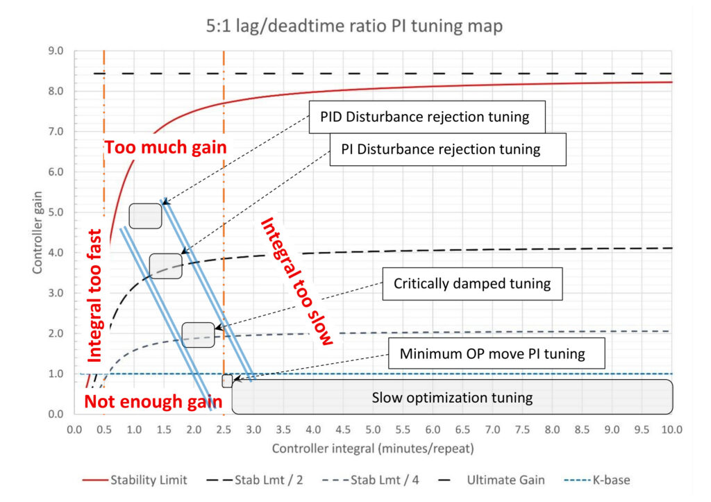
Figure 1: Self-limiting process PI controller tuning map. Lag/deadtime ratio = 5:1. K_p = 1.0, T₁ = 150 seconds, D_t = 30 seconds. Courtesy: Ed Bullerdiek, retired control engineer

In Figure 1 the double blue lines set a boundary on controller gain and integral tuning constants that will likely work well for this process. The windows tell us where specific types of controller performance will be found, although the best blend is the one that gives you the best performance for your specific situation whether that is inside one of the windows or not. The red labels tell you where you are if you are using heuristic methods to tune this controller. PID spotlight parts 9 and 10 cover pattern recognition and what to do when you identify that the controller’s (for example) integral is set too slow.

How can I find the PID controller performance windows?

In PID spotlight part 26 we learned that:

• The locations of the performance windows could change relative to each other depending on the lag/deadtime ratio of the process.
• The disturbance rejection and critically damped windows are not available for deadtime dominant processes.
• Some common published loop tuning methods do not work well at all lag/deadtime ratios.

This points out the need for estimation methods for each of the performance windows and the range of applicability. The following calculations were developed using heuristic methods to find optimal tuning for each of the performance windows across lag/deadtime ratios from 100:1 down to 1:100 followed by curve fitting the results. The caveat is these calculations reflect my personal preferences, which is true for all the authors of the 400+ tuning methods (and yes, of course I think mine are better. But I encourage you to find what works best for you.)

Finding the disturbance rejection tuning window

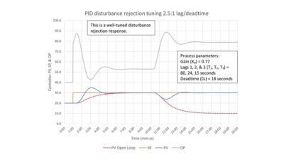
The calculations in Table 1 can be used to calculate the approximate midpoint of the PI and PID disturbance rejection windows from open loop step test data. The PI disturbance rejection tuning calculations will work for lag/deadtime (L/D) ratios from 100:1 down to 1:4. The PID disturbance rejection calculation is good for L/D ratios from 100:1 down to 1:1.

Derivative cannot be used on a true first order plus deadtime (FO+D_t) process because derivative behaves badly on sudden changes in direction. Very high lag/deadtime ratio processes may be effectively FO+D_t. You may not be able to use PID disturbance rejection tuning. Fortunately at very high L/D ratios disturbance rejection is very good for PI only tuning.

Regardless, if you are really trying to squeeze that last bit of performance derivative can be set as high as one-tenth of the integral (T_d = T_i/10) constant at L/D ratios from 100:1 down to 30:1. For L/D ratios between 4:1 and 1:1 setting derivative to one-fourth of the integral (T_d = T_i/4) constant usually works well, and between 30:1 and 4:1 a linear interpolation {T_i/(3.08+0.23*T₁/D_t)} provides a good starting point. Regardless of L/D ratio, if the process is close to a true FO+D_t process, you may have to use heuristics to reduce derivative and possibly controller gain and integral.

The general rule for tuning applies to these and the tuning calculations that follow: The process you encounter will likely not be first order plus deadtime. It may actually have complex dynamics that look kind of like first order. You may be trying to fit a sort of round peg into a sort of square hole and find that you have to use heuristics to get the performance you are looking for.

Finding the critically damped tuning window

Table 2 calculates controller gain and integral constants that will provide slightly aggressive critically damped tuning. In the interest of getting consistent time to setpoint measurements across all lag/deadtime ratios, I aimed for 5% overshoot (a 10% setpoint change results in the process variable overshooting the new setpoint by 0.5%.) at every ratio tuned. This will also result in the controller output overshooting its final value by 5% when a disturbance occurs.

Should you desire less overshoot increase (slow down) the integral time. For high L/D ratios (when deadtime doesn’t affect integral) setting integral equal to the lag time (T_i = T₁) will result in no overshoot. Setting T_i = 0.71*T₁ results in 1% overshoot; T_i = 0.32*T₁ results in 5% overshoot, and T_i = 0.186*T₁ results in 10% overshoot. Once deadtime becomes prominent these relationships break down, but work directionally if you need to make adjustments.

These calculations are good for L/D ratios from 100:1 down to 1:5, however at an L/D ratio below 1:1 you would be better served using the minimum controller output movement tuning calculations below.

Finding the minimum controller output movement tuning window

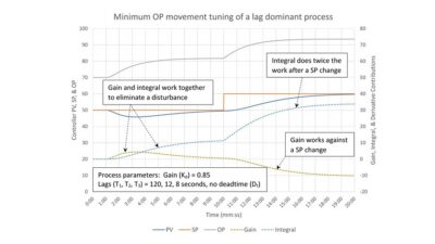
Table 3 calculates the controller gain and integral that will result in minimum controller output movement when the controller setpoint is changed. These calculations are valid for the full lag/deadtime ratio from 100:1 down to 1:100. Below an L/D ratio of 1:4 these are the only calculations that will provide good control (with the standard disclaimer that you may still need to do some trimming).

In reality, you will never use this calculation for any L/D ratio greater than 2:1. You can set the controller gain equal to the baseline controller gain (K = K_base) and integral equal to the lag time (T_i = T₁) with very little impact of performance. (Why overthink it?)

Estimating ultimate gain (K_u) and natural period (P_n)

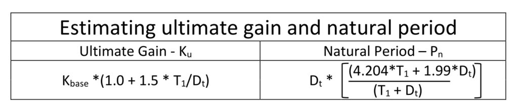
Table 4: Estimating ultimate controller gain (K_u) and natural period (P_n) from open loop step test data. Courtesy: Ed Bullerdiek, retired control engineer

In the event you want to use a closed loop tuning method but only have open loop step test data, you can use the calculations in Table 4 to estimate controller ultimate gain (K_u) and natural period (P_n). One of the interesting things that emerged from this exercise was finding out that natural period is not always four times the deadtime. This is only true at high lag/deadtime ratios. Natural period is two times deadtime for deadtime dominant processes and about three times deadtime at an L/D ratio of 1:1.

Charting the data

Following are charts showing how controller gain and integral change for the controller performance windows across the full range of expected lag/deadtime ratios.

Controller gain multiplier:

In figures 2 and 3 the vertical scale is the controller gain multiplier (K_x), the value you must multiply the baseline controller gain (K_base) by to get the final controller gain (K).

K = K_x * K_base

Figures 2 and 3 include plots of the ultimate controller gain (K_u), PID and PI disturbance rejection gain (0.60 * K_u and 0.45 * K_u respectively), critically damped controller gain (0.25 * K_u) and minimum control output movement gain (always less than 1.0 * K_base).

Figure 2: Map of baseline controller gain (K_base) multipliers for disturbance rejection, critically damped and minimum OP movement tuning based on lag/deadtime ratio for self-limiting processes. Courtesy: Ed Bullerdiek, retired control engineer

Figure 2 is the fully expanded version of Figure 1 from PID spotlight part 6 which is where we first looked at the relationship among lag/deadtime ratio, controller tuning and controller performance. The quick summary of that article is when the lag/deadtime ratio is high, tuning is easy and disturbance rejection very effective. As the ratio drops, controller tuning becomes more difficult, and performance degrades to the point where disturbances are fully expressed and persistent.

We can see from Figure 2 why tuning in the lag dominant area is easy. At a 100:1 lag/deadtime ratio you can set the controller gain up to 150 times the baseline controller gain and while going above 67 is probably not a great idea that still leaves you a lot of room to work. Even at 10:1 there is ample room to work with controller gain.

However, as we get to lower lag/deadtime ratios ultimate gain drops, which constrains the controller gain to the point where we need to take a closer look at what’s going on (Figure 3).

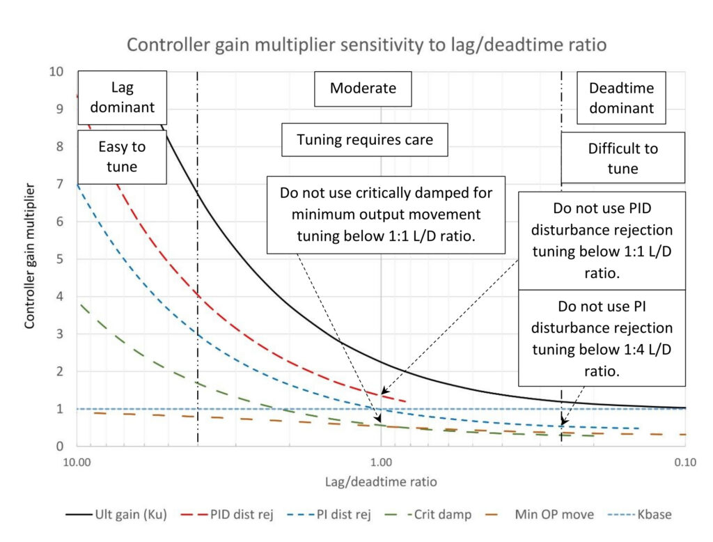
Figure 3: Map of baseline controller gain (K_base) multipliers for PID and PI disturbance rejection, critically damped and minimum OP movement tuning based on lag/deadtime ratio for self-limiting processes. Courtesy: Ed Bullerdiek, retired control engineer

Figure 3 three is a close up of when the lag/deadtime ratio transitions from lag/dominant to deadtime dominant. The important transition points are:

• Lag/deadtime ratio < 1:1:
• Do not use PID disturbance rejection tuning.
• Substitute minimum OP movement tuning for critically damped tuning.
• Lag/deadtime ratio < 1:4:
• Do not use PI disturbance rejection tuning.

Below a 1:4 lag/deadtime ratio only minimum OP movement tuning will work effectively. The other tuning methods become oscillatory and ineffective.

Let’s take a moment to appreciate the work of Ziegler and Nichols on controller gain. I started heuristic tuning for PID and PI disturbance rejection tuning from Z-N’s correlation to ultimate controller gain (K_u) and never drifted far from it regardless of lag/deadtime ratio. Critically damped tuning controller gain settled in at 0.25 * K_u for all lag/deadtime ratios also. Ultimate controller gain is very easy to estimate for all lag/deadtime ratios so the individual gain calculations were no more difficult that multiplying 0.6, 0.45 and 0.25 through the ultimate controller gain calculation.

Obviously, the minimum controller output movement correlation is very different as the performance goal for this tuning is very different. And the integral correlations weren’t as easy.

Controller integral multiplier:

The vertical scale in figures 4 and 5 is the controller integral multiplier (T_iX), the value you must multiply the process deadtime (D_t) by to get the final integral (T_i).

T_i = T_iX * D_t

In contrast to the controller gain multiplier plots on these charts, bigger is slower. There is no equivalent to ultimate controller gain (K_u) as no matter how fast you set integral, the controller can always be made stable if you turn the controller gain down far enough. The process lag is added as a reference as rarely is integral much bigger than the process lag.

Figures 4 and 5 include plots of:

• Lag: This is the process lag.
• PID dist rej: The PID disturbance rejection integral constant multiplier.
• PI dist rej: The disturbance rejection integral constant multiplier.
• Crit damp: The critically damped (setpoint following) integral constant multiplier.
• Min OP move: The minimum controller output movement integral constant multiplier.
• Nat per (P_n): The natural period (P_n) multiplier.

The PID and PI disturbance rejection, critically damped and natural period curves are all hyperbolic curves requiring complex curve fits. The logarithmic plot obscures this by bending them into what appears to be an S-shape. The minimum OP move curve is simple as it lays on top of the process lag until deadtime becomes significant.

Figure 4: Map of integral by deadtime (D_t) multipliers for disturbance rejection, critically damped and minimum OP movement tuning based on lag/deadtime ratio for self-limiting processes. Courtesy: Ed Bullerdiek, retired control engineer

In Figure 4 we can see how disturbance rejection, critically damped and minimum controller output movement tuning diverge at higher lag/deadtime ratios. The integral constant for disturbance rejection tuning remains close to the process deadtime regardless of the lag/deadtime ratio. This tells us that any tuning method that sets integral equal to the process lag will perform poorly at disturbance rejection at high L/D ratios.

Critically damped tuning naturally falls between the deadtime and process lag at high L/D ratios. As stated above the choice of integral constant can be moved up (slower) or down (faster) depending on how aggressive the tuning needs to be.

Integral for minimum OP movement tuning matches the process lag at high L/D ratios as this is the setting that results in no overshoot or undershoot on controller output movement.

Figure 5: Map of integral by deadtime (D_t) multipliers for disturbance rejection, critically damped and minimum OP movement tuning based on lag/deadtime ratio for self-limiting processes. Courtesy: Ed Bullerdiek, retired control engineer

Figure 5 is a close up of the lower integral multiplier range so that we can get a closer look at the impact of increasing deadtime on controller tuning. Several things stand out:

• The natural period (P_n) drops from slightly over 4.0 at a 10:1 lag/deadtime ratio to 2.0 at a 1:30 L/D ratio. Various publications have stated that the natural period can be estimated at either three or four times deadtime, which begs the question: Which is true? The true answer is, “It depends.”
• The PID and PI disturbance rejection integral lines cross over the critically damped and minimum controller output integral lines between a L/D ratios of 1 and 2. Presumably the higher controller gain constrains how much integral can be applied.
• The critically damped integral line crosses the process lag at about a 1.05 L/D ratio. At this point the integral tuning is now slower than the process lag.
• The minimum controller output movement integral line diverges from the process lag as the deadtime increases.

All of these expose the increasing impact deadtime is having on controller tuning and performance. Once controller gain has dropped below baseline controller gain, and integral is slower than the process lag, we have transitioned to a point where the PID controller can no longer respond to disturbances well or execute setpoint changes crisply. All of this occurs around a lag/deadtime ratio of 1:1.

Ed Bullerdiek is a retired control engineer with 37 years of process control experience in petroleum refining and oil production. Send comments and questions to [email protected]. Edited by Mark T. Hoske, editor-in-chief, Control Engineering, WTWH Media, [email protected].

Keywords

Proportional-integral-derivative, PID tutorial

Learning objectives

• Know how to calculate tuning constants for PID and PI disturbance rejection, critically damped and minimum output movement tuning from open loop step test data.
• Know how to estimate controller ultimate gain (K_u) and natural period (P_n) from open loop step test data for use in closed loop tuning methods.
• Understand the ranges of applicability for these tuning calculations.
• Understand how lower lag/deadtime ratios compress the controller gain and integral tuning windows.

Consider this

After you determine the performance requirement for your PID controller the appropriate tuning constant calculations can get you started in the right direction. However, these are just guidelines, not final answers.

You also might like

PID series from Ed Bullerdiek, retired control engineer

PID Spotlight, part 1: Three reasons to tune control loops: Safety, profit, energy efficiency

PID spotlight, part 2: Know these 13 terms, interactions

PID spotlight, part 3: How to select one of four process responses

PID spotlight, part 4: How to balance PID control for a self-limiting process

PID spotlight, part 5: What does good and bad controller tuning look like?

PID spotlight, part 6: Deadtime? How to boost controller performance anyway

PID spotlight, part 7: Open-loop tuning of a self-limiting process

PID spotlight, part 8: Closed-loop tuning for self-limiting processes

PID spotlight, part 9: Heuristic tuning for a self-limiting process (part A on heuristic tuning)

PID spotlight, part 10: Heuristic tuning in a self-limiting process

PID spotlight, part 11: How a PID controller works with an integrating process

PID spotlight, part 12: What does good and bad controller tuning look like?

PID spotlight, part 13: Deadtime: what’s the best that I can do?

PID spotlight, part 14: Open loop tuning of an integrating process

PID spotlight, part 15: Open loop tuning of near integrating processes

PID spotlight, part 16: Closed loop tuning of an integrating process

PID spotlight, part 17: Heuristic tuning of an integrating processes

PID spotlight, part 18: Identifying control valve performance problems

PID spotlight, part 19: PID controller tuning mechanics

PID spotlight, part 20: Tuning with bad valves

PID spotlight, part 21: Noise: Can I tune around it?

PID spotlight, part 22: Can I tune a noisy PID controller?

PID spotlight, part 23: Filtering noise for better PID control

PID spotlight: part 24: How do I tune PID controllers during a new unit startup?

PID spotlight, part 25: Navigating PID controller tuning

PID spotlight, part 26: How fast should I tune my PID controller?

More on PID and advanced process control from Control Engineering

https://www.controleng.com/control-systems/pid-apc