How do I prevent process noise or a sticking control valve from disturbing the rest of my process? What works and how should it be set up?
Insights about PID gap control
- Setpoint (SP) gap action can reduce the spread of disturbances to the rest of the process caused by process noise or a sticking control valve.
- The SP notch and floating SP gap algorithms work best for reducing the effect of process noise and sticking control valves.
- The SP V-notch and error squared gap algorithms are less effective at reducing the effect of noise and should not be used to manage a sticking control valve.
One of the top rules for reducing variability in a process is to not have the control system add unwanted variability. In the articles on bad control valves and process noise we learned that process noise and bad valves can cause unwanted control valve movement, which will add variability to the process. In the case of process noise, filtering and judicious tuning changes can help, but cannot entirely remove unwanted valve movement. Bad control valves cause limit cycling, which cannot be eliminated by controller tuning, adding unwanted variability to the process. (If you haven’t already, please read PID spotlight parts 18 and 20 on bad control valves and PID spotlight parts 21 through 23 on process noise; link to prior articles at bottom.)
Setpoint (SP) gap action can be used to reduce, but not fully eliminate, the addition of unwanted variability to the process by process noise or a bad valve. We also learned that process noise and bad valves can complicate loop tuning efforts, increasing the chance of inadvertently installing unstable tuning constants. As we learned in PID spotlight part 32, adding SP gap action can help stabilize controllers with overly aggressive tuning, which buys us room for mistakes when tuning these controllers.
Managing process noise with SP gap action
Generally, adding SP gap action should be considered the last option for managing process noise. Mild noise should be handled through filtering. Significant noise can be handled with heavy filtering if the process is slow enough and slow tuning is acceptable. Candidate processes for SP gap action will be very noisy, fast and generally require reasonably fast control.
Tuning noisy processes requires the elimination of derivative and the reduction of controller gain to minimize the passthrough of noise to the controller output (OP). Integral is sped up to attempt to recapture some of the performance of the controller, but at the risk of creating oscillation due to excessive integral speed. While an SP gap can increase apparent deadtime, it will still allow speeding up integral while maintaining controller stability.
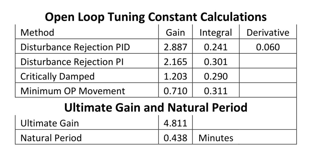
We are going to work with a fairly fast process with a process gain (Kp) of 1.0, two lags of 10 seconds, and a deadtime of 5 seconds. This results in an overall lag of 18.7 seconds and an apparent deadtime of 7.3 seconds for a calculated lag/deadtime (L/D) ratio of 2.54:1. The table summarizes the calculated tuning constants, estimated ultimate gain and natural period. (And, as always, real world data will never be this precise.)
Planning to manage process noise with SP gap action
The first step in managing a noisy process is setting up the noise filter. This is a fast process, and we need to have reasonably aggressive control, therefore the noise filter should be limited to no more than 12 seconds. More will do little to reduce the noise signal while also adversely affecting how fast this controller can be tuned (see PID spotlight part 23).
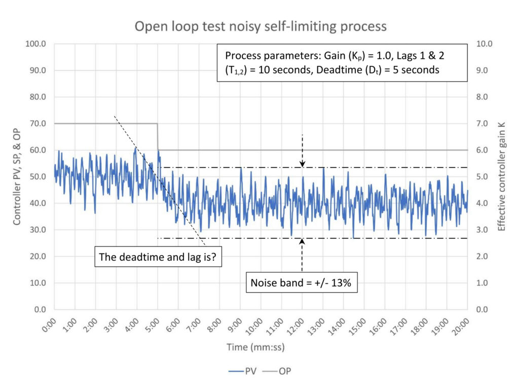
Figure 1 shows us what we are up against in trying to tune this controller. The process has a very wide noise band, nominally about ±13% around the average process variable (PV) value, and the noise doesn’t appear to be white or to have any specific cycle. Based on the step test at the 5-minute mark the process appears to respond quickly to the change in controller output, but any guess at the deadtime and process lag is just that – a guess. Increasing the OP step size might help, but we are already up against the step size limit requested by the process operator. Adding a 6 second filter should get us about a 70% reduction in noise (the control system filter is entered in minutes; 0.1 minutes is a quick and easy entry. If your system measures filter time in seconds, then 5 or 10 seconds will work. Do not overthink this.)
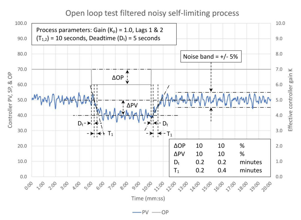
A 6 second filter has been added in Figure 2. The visual span of the noise has been reduced to about ±5%, which is approximately a 60% reduction in the noise signal. Because this is not true white noise, the result is not unexpected. The open loop step test results are somewhat ambiguous, but we know that since this is a noisy process, we are going to use a low controller gain and a very fast integral time. The first step test in Figure 2 gives us the lowest recommended controller gain and fastest recommended integral time. These are:
K = 0.542 (minimum OP movement)
Ti = 0.223 (critically damped)
In deference to the uncertainty in the test results we will round these to K = 0.5 and Ti = 0.25 just to start on the safe side. Note that the true tuning constants in Table 1 would allow a much larger controller gain for minimum OP movement tuning (0.71) and roughly the same integral (0.24). However, because we need to reduce the OP movement, we would have likely still reduced the controller gain to 0.5. In this case, it appears the noise hasn’t lead our test results too far astray.
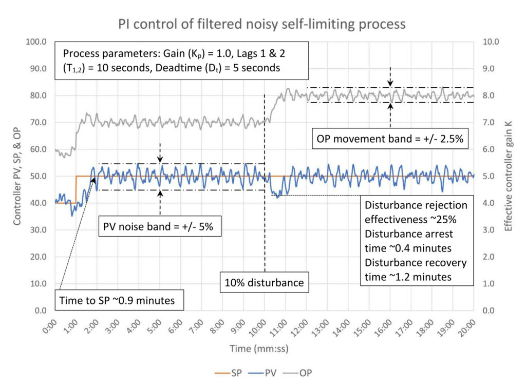
Figure 3 shows how this first attempt at tuning worked out. The first thing to note is the process variable noise band hasn’t gotten any smaller. A relatively slow PID controller cannot reduce process noise. But the PV noise band hasn’t gotten larger, which a poorly tuned PID controller can do. The good news is the noise isn’t any worse.
Next, the controller output movement band is ± 2.5%. This is as expected for a controller gain of 0.5; it should be half the PV noise band and, since this is a reverse acting controller, the mirror image of the PV noise band.
The estimated controller performance is in line with the expected performance for a process with a 1:1 L/D ratio tuned for minimum OP movement performance. (The true process L/D ratio is 2.5:1, but the tuning was set using the most conservative L/D ratio from the testing in Figure 2, which is 1:1.) Ideally, the disturbance rejection effectiveness could be as high as 65%, but this would require considerably raising controller gain and adding derivative. Given the amount of noise, this is simply not possible, which points to the problem with process noise: It puts a hard upper clamp on what we can do to get better performance.
Regardless, for this specific process, we still have a requirement to minimize controller output movement to prevent spreading a localized phenomenon, process noise, to the rest of the process through control valve movement. Reducing OP movement can be done using a SP gap, which allows the controller to ignore PV movement within the noise band but still respond to setpoint changes and disturbances. This will also allow us to speed up the controller tuning some, but this will likely not improve overall controller performance.
Which SP gap algorithm you use depends on the details of the PID controller algorithm. If you haven’t already, please read PID spotlight parts 31 and 32 for details on SP gap algorithm implementation, how to determine which PID algorithm your system uses and which SP gap algorithm should be used with which PID algorithm.
Notch gap setup for a classical PID controller; velocity form
The objective of applying a notch gap to a noisy process is to stop the controller output from moving when the process is stable and centered on the setpoint. To do this the high and low gap limits are set at the noise limits; in this example plus and minus 5%. Then the gap gain is set to zero. We will start with the tuning from Figure 3, but with the understanding that we will very likely make it more aggressive.
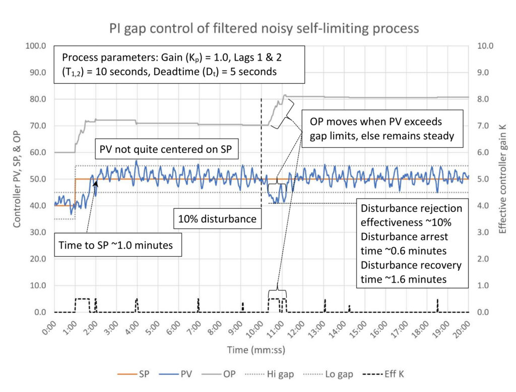
The effect of adding SP gap action is shown in Figure 4. Adding the SP gap had the desired effect of largely stopping OP movement except after the SP change at the 1-minute mark and the disturbance at the 10-minute mark. However, after adding the gap, the controller performance measures all got worse (as expected). There are also some PV drift issues that suggest tightening up the gap, but we will save that for later.
Since there is no sign of overshoot on either the SP change or the disturbance there should be some room to speed up the controller tuning. For noise control we want the controller to operate almost exclusively on integral action. Heuristic tuning rules suggest we should speed up the integral by cutting the integral constant by 25-50%. To speed things along, let’s cut integral by 50% to 0.125 minutes/repeat. This is twice as fast as any of the calculated integral constants for the true process or any of the estimates from Figure 2. Regardless, since there is no evidence of overshoot, this should be safe.
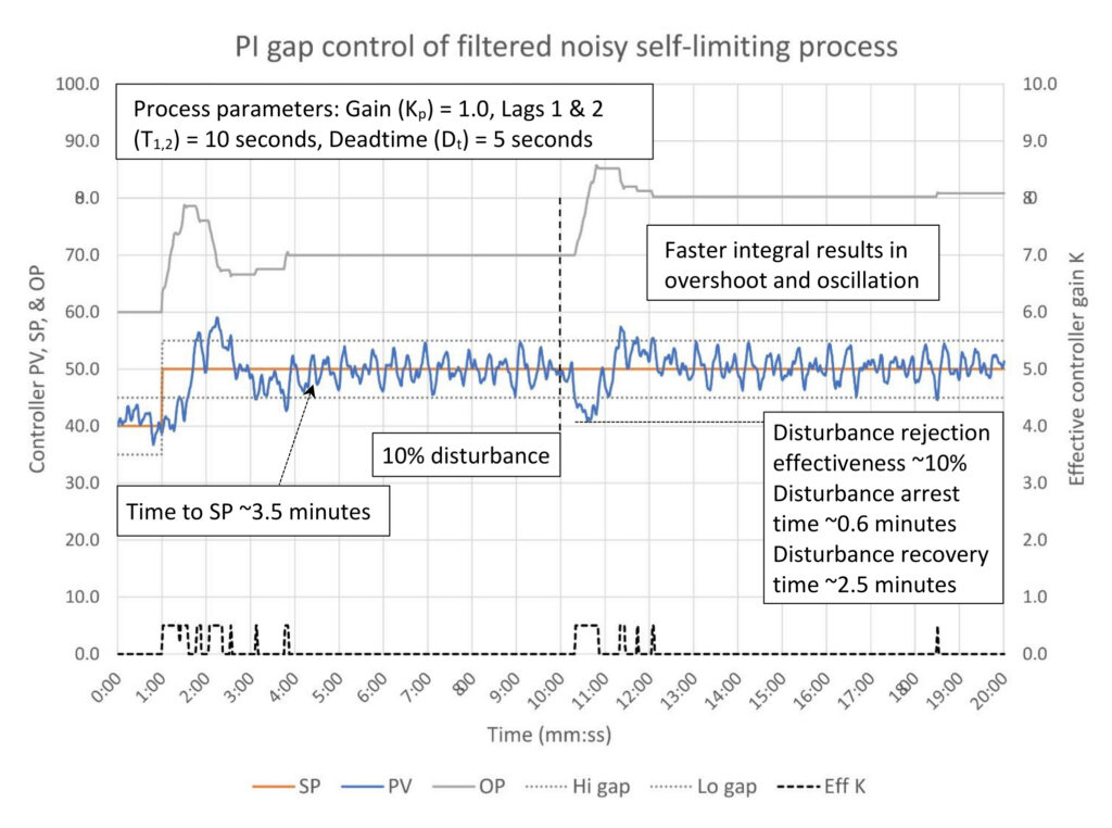
Speeding up the integral did result in some overshoot and oscillation after the SP change and overshoot after the disturbance (Figure 5). However, it does not appear to have helped the controller performance. The disturbance recovery time and time to setpoint both get penalized because of the overshoot. The OP did land on its final value more rapidly, minimizing the PV time off setpoint relative to Figure 4, but this may just be good luck.
Depending on preferences, the controller tuning could be left here, or the next step may be to split the difference on the integral constant and perhaps reduce the gap size to ± 4%. (A side investigation showed that tuning had little impact on controller performance for smaller disturbances, 10% or so, but the impact of a large, say 40%, disturbance can be reduced by higher controller gain, as expected. However, a controller gain much higher than critically damped (1.2) will cause excessive oscillation. Since the objective here is to reduce controller output movement, controller gain should be limited.)
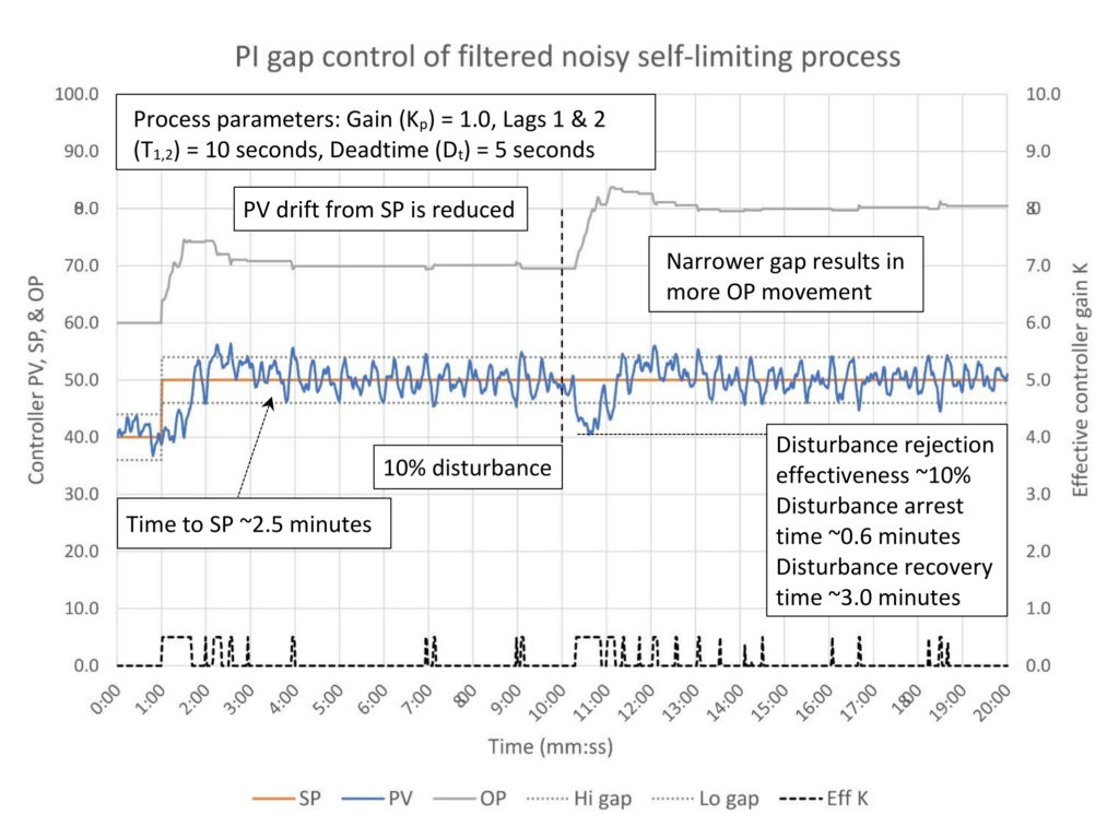
In Figure 6 integral is slowed down to 0.19 minutes/repeat and the SP gap is narrowed to ± 4% to eliminate oscillation, lower overshoot and reduce PV drift from setpoint. It appears all these goals have been met. Controller performance is not significantly changed, nor was this expected. There is, however, more OP movement, which depending on process needs may or may not be acceptable.
V-notch gap setup for a classical PID controller; positional form
Unless you are willing to engage in some customization a commercial V-notch filter will not provide a band where the controller gain is zero. The controller gain when the error is zero (Knotch) will be zero. The only question will be how big the controller gain slope will be (Kslope). For the notch SP gap application above a controller gain of 0.5 was selected for any PV excursion outside a ±5% band from setpoint. A good starting point for the gain slope would be for the controller gain to equal 0.5 when the PV error is 5%, the edge of the noise band. Since the units on Kslope are ΔK/Δ10% error and Knotch is zero, by substituting and rearranging the V-notch gain calculation:
K = ABS(Error)*Kslope/10 + Knotch
0.5 = 5.0*Kslope/10 + 0
Kslope = (0.5 / 5.0) * 10
Kslope = 1.0
That looks deceptively simple.
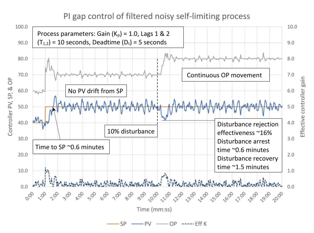
When comparing the V-notch gap controller performance in Figure 7 to the notch gap performance in Figure 4, the first thing that stands out is there is continuous controller output movement. This is expected because unless the error is zero there is always some gain. However, compared to the controller without gap action in Figure 3, there is quite a bit less OP movement. As expected, the V-notch controller performance is little different from the notch controller in terms of disturbance rejection and arrest time, etc. There is no problem with PV drift from SP, unlike the notch gap algorithm, again because there is always some control action when the PV is not on SP.
While this is not shown, speeding up integral to 0.125 minutes/repeat is unstable.
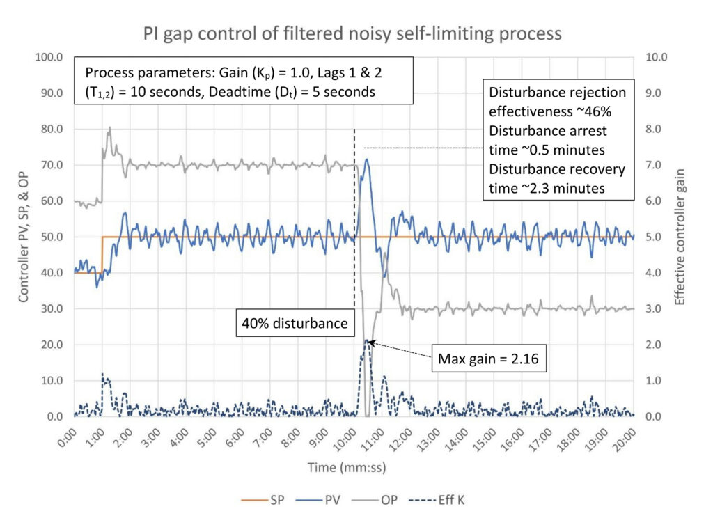
The one concern with the V-notch gap algorithm is controller stability when a large disturbance occurs because the controller gain continues to increase with error. Figure 8 shows the controller response to a 40% disturbance. The controller response is stable even though the controller gain peaks at 2.16, however, the controller output does saturate. Disturbance rejection effectiveness climbs to 46%, which is good for the 1:1 L/D ratio estimated from the step test in Figure 2.
Depending on preferences, the OP movement might still be considered excessive. Kslope could be reduced to 0.75 or even 0.5 to reduce OP movement, but the tradeoff is reduced disturbance effectiveness when large disturbances occur.
Error squared gap setup for a parallel PID controller
The error squared gap algorithm’s behavior is nearly identical to the V-notch algorithm when Knotch is zero. The one difference is the error squared gap algorithm presented here puts a cap on the controller gain, whereas the V-notch algorithm does not. Therefore, there is no concern about controller stability when very large disturbances occur. The setup is different in that you need to set the controller tuning and the width of the gap, which in this case will be:
K = 0.5
Ti = 2 repeats/minute
SD = 5%
Note that the integral constant is expressed in the units used by a parallel PID algorithm.
Of course, these tuning constants are a starting point. You may choose a higher controller gain and/or faster integral along with a wider scaling divisor (SD) for more aggressive control. Or you may choose to set controller gain to zero and use integral only control. Regardless, no figures are included as they would be redundant to the V-notch gap algorithm discussion.
Floating setpoint gap setup for a parallel PID controller
The assumed starting tuning constants for a parallel PID controller using the floating SP gap algorithm is the equivalent tuning used in the notch SP gap classical PID algorithm above; K = 0.5, Ti = 2 repeats/minute and the gap is ±5%.
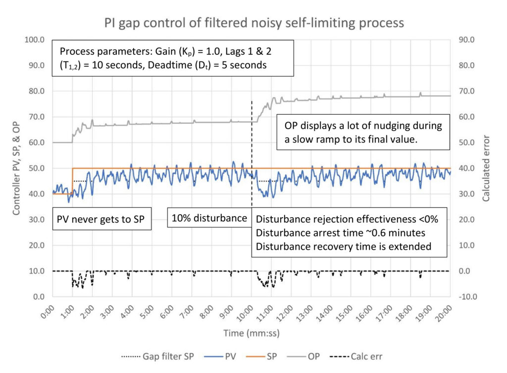
The controller response in Figure 9 looks nothing like controller response in Figure 4. Heuristics indicate that integral is far too slow using the floating SP gap algorithm, whereas it is perhaps a little fast in the notch gap algorithm used in Figure 4. Digging into the details of the two algorithms, the integral calculation in the notch gap algorithm measures error from the setpoint. Thus, if the gap is 5%, but the error is 10%, the integral calculation is based on the error of 10%. In this same situation, the floating SP gap algorithm presents an error of 5% to the PID controller, and therefore the integral calculation is based on an error of 5%. This considerably reduces the speed of the integral action, nearly eliminating it for small excursions outside the gap.
The notch gap algorithm, by calculating integral from the setpoint, makes using standard tuning calculation methods more consistent. The floating SP algorithm complicates tuning for these specific situations. Integral must be sped up; heuristic methods will be required, and we must pay much closer attention to the maximum size of potential upsets.
Heuristics in this instance would suggest doubling integral speed to Ti = 4.0 repeats/minute.
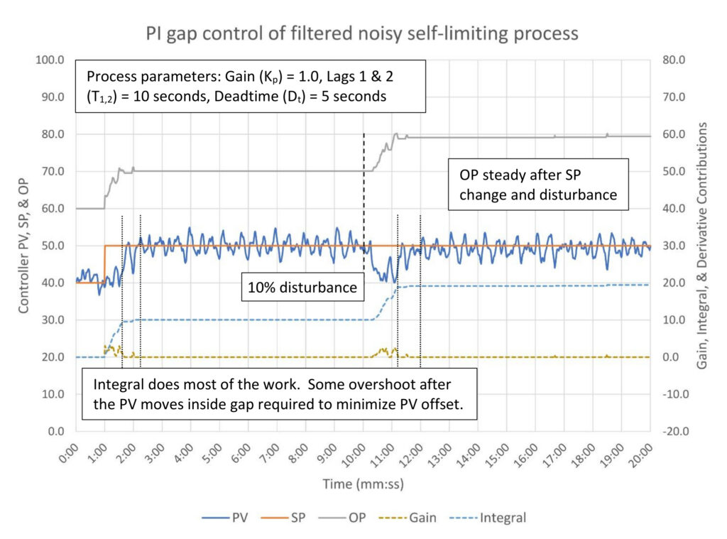
Speeding up the integral addressed the failure of the PV to reach setpoint (Figure 10), which also reduced the number of nudges that occur when the PV reaches the edge of the gap. The controller gain and integral contributions were included in Figure 10 to show how dominant the integral action is relative to controller gain. Dashed lines were added between when the integral stopped moving after both the SP change and the disturbance to highlight how the integral must cause some overshoot to get the PV close to setpoint. This additional integral could lead to instability if a large disturbance occurs.
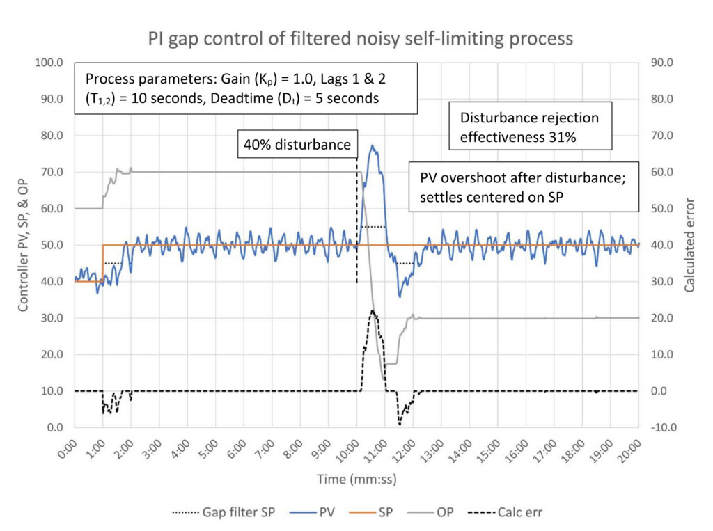
A 40% disturbance was added in Figure 11 to test controller stability. The PV does overshoot the setpoint after the disturbance, but there are no following oscillations. As was demonstrated in PID spotlight part 32, disturbance rejection effectiveness does improve with larger disturbances when gap control is used. In this case, disturbance rejection effectiveness is 31% for a 40% disturbance. This is not outstanding compared to what should be possible with this process, which shows again the problems process noise causes.
What if we used more filtering?
No figures are provided, but increasing the filter time to 12 seconds was tested. The additional filtering reduces the PV noise band to ±3%, a 40% reduction relative to the ±6 second filter constant. However, the added apparent deadtime required slowing the integral constant down 40%, resulting in slower overall control. This points out the tradeoffs between filtering, tuning and overall controller performance when we encounter process noise. There is no one good answer, only a series of tradeoffs that can result in unique solutions to the different problems you will encounter.
Managing a bad control valve with SP gap action
A sticking control valve will result in a continuous valve position limit cycle when a controller is in auto. This will cause the process variable, and the rest of the process, to cycle with the control valve. Tuning alone cannot fix this. The only choice when using tuning alone is whether the cycle is fast or slow. The ideal solution is to fix the valve, but this may have to wait. The next option is to install a positioner, which is expensive and also takes time. For the slow processes typical in refining, cascading the slow process to a flow controller usually helps, but requires the presence of a flow instrument.
If none of these solutions are available, then using SP gap action can be a suitable stopgap. The tradeoff is that to achieve stability you must be willing to accept that the process variable will be off setpoint for extended periods of time. This can be the lesser of two evils in many processes.
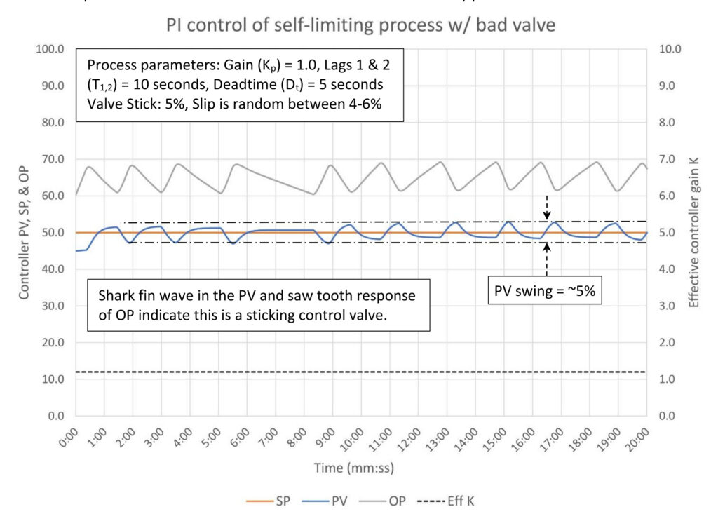
Setting up a SP gap controller for a sticking valve follows the same method used for a noisy process; set the gap width a little bit wider than the PV limit cycle (think of it as the noise band). Figure 12 is an example of a process variable with a shark fin wave and the controller output with the saw tooth wave, which characterizes a sticking control valve. Since our goal is to stop the limit cycle, the SP gap must be set just slightly wider than the PV swing. In Figure 12, the swing appears to be about 5%, which means setting the controller gap at ±3% around the setpoint. Of course, this means we must be willing to let the PV run for extended periods of time at up to 3% from setpoint.
Notch gap setup for a classical PID controller; velocity form
For an SP notch gap, the setup is straight forward: Set the high and low gap limits at 3% and the gap gain multiplier at zero. This should capture the control valve at a position where the PV is inside the gap limits.
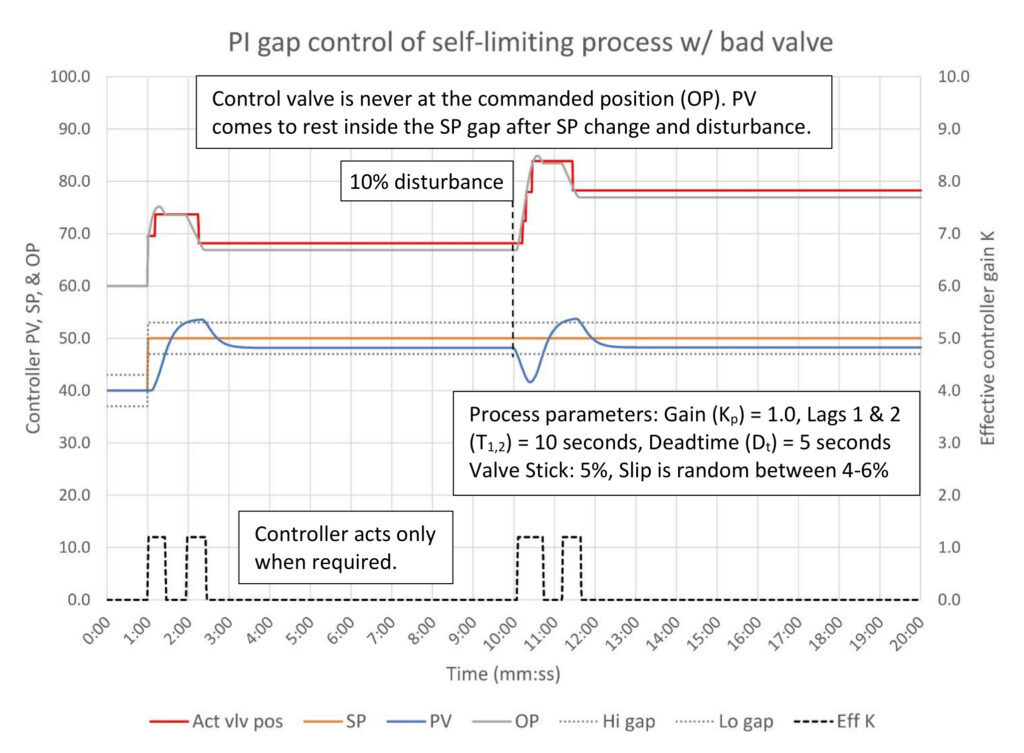
The controller in Figure 13 is tuned for critically damped performance. One of the lessons from the prior review of tuning with a bad control valve is that a sticking valve can create unpredictable deadtime, which can result in instability when aggressive tuning is used. Adding a SP gap can help some, but the recommendation to limit controller aggressiveness still applies.
Adding the SP gap achieved our goal of stopping the limit cycle, but with the side effect of allowing the PV to deviate from SP for potentially an unlimited amount of time. Note that after the SP change and disturbance, the PV did overshoot the edge of the gap, and controller had to make a correction. If this behavior persists lowering controller gain will help. The actual valve position is included to show that except by happy accident the actual valve position never matches the commanded position.
Once acceptable performance is achieved, there is little point in trying to optimize controller tuning. Valve stick/slip performance can be highly variable. It is best to write a work order to fix the valve and wait for repairs.
V-notch gap or error squared gap non-performance
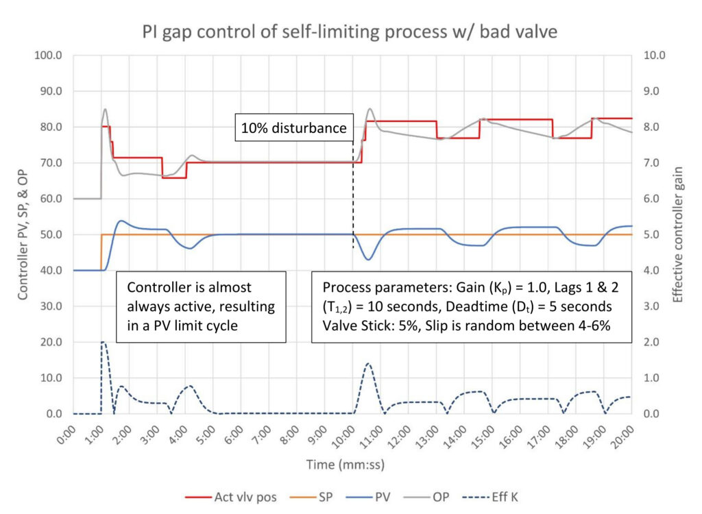
The V-notch and error squared SP gap algorithms are not recommended to manage bad valves. Because there is always some controller movement when the error is not zero with either algorithm, integral action will ramp the controller output until the valve moves. Figure 14 is an example of this using the V-notch algorithm. Briefly after the SP change, the PV did match the SP, but then the disturbance resulted in a continuous limit cycle. The effective controller gain trend tells the story; with the exception of when the PV crosses over, the SP the controller is always active. No figure for the error squared SP gap algorithm is included, but it performs the same way.
Floating setpoint gap setup for a parallel PID controller
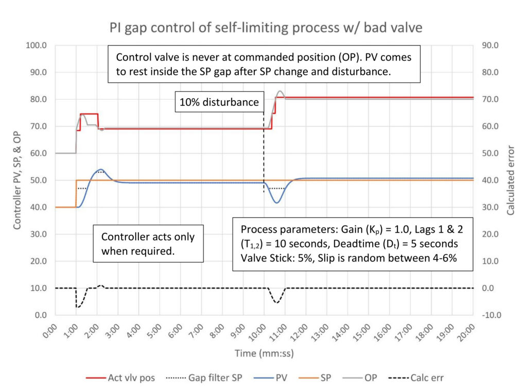
The controller in Figure 15 is tuned for critically damped response. Remember that for the parallel PID algorithm a bigger integral constant is faster. The response is very similar to the SP notch gap algorithm applied to a classical PID controller. There are fewer problems with PV overshoot due to differences in the gap algorithm.
Reflections on gap control
SP gap control is an overlooked topic. It is rarely discussed, and when it is discussed, the focus is on level surge control (which will be discussed later) or managing sticking control valves. Applications here are presented as ideas to stimulate creative thought about how to manage controller gain to meet process objectives.
One of the repeated themes in this series is to test your system. Unfortunately, there is no way to get around the fact that success requires knowing your system’s details. This introduces a level of complexity that gap controller discussions gloss over. Controller gain modification can be a very useful tool to improve performance when applied properly, but applying a gap algorithm that isn’t compatible with your system will result in failure.
Finally, if you are willing to do some customization, these articles provide some application suggestions, and you are encouraged to look for more. As always, some planning, documentation and simulation work are recommended before putting anything in service.
Ed Bullerdiek is a retired control engineer with 37 years of process control experience in petroleum refining and oil production. Send comments and questions to [email protected]. Edited by Mark T. Hoske, editor-in-chief, Control Engineering, Arrowfly, [email protected].
Keywords
Proportional-integral-derivative, PID tutorial
Learning objectives
- Understand that a setpoint gap can reduce control valve movement, and thus disturbances to the rest of the process, when there is process noise or a sticking control valve.
- Know how to select and set up a setpoint gap algorithm for process noise management.
- Know how to select and set up a setpoint gap algorithm when the control valve sticks.
Consider this
Thinking about setpoint gap may stimulate creative thoughts about how to manage controller gain to meet process objectives.
You also might like
PID series from Ed Bullerdiek, retired control engineer
PID Spotlight, part 1: Three reasons to tune control loops: Safety, profit, energy efficiency
PID spotlight, part 2: Know these 13 terms, interactions
PID spotlight, part 3: How to select one of four process responses
PID spotlight, part 4: How to balance PID control for a self-limiting process
PID spotlight, part 5: What does good and bad controller tuning look like?
PID spotlight, part 6: Deadtime? How to boost controller performance anyway
PID spotlight, part 7: Open-loop tuning of a self-limiting process
PID spotlight, part 8: Closed-loop tuning for self-limiting processes
PID spotlight, part 9: Heuristic tuning for a self-limiting process (part A on heuristic tuning)
PID spotlight, part 10: Heuristic tuning in a self-limiting process
PID spotlight, part 11: How a PID controller works with an integrating process
PID spotlight, part 12: What does good and bad controller tuning look like?
PID spotlight, part 13: Deadtime: what’s the best that I can do?
PID spotlight, part 14: Open loop tuning of an integrating process
PID spotlight, part 15: Open loop tuning of near integrating processes
PID spotlight, part 16: Closed loop tuning of an integrating process
PID spotlight, part 17: Heuristic tuning of an integrating processes
PID spotlight, part 18: Identifying control valve performance problems
PID spotlight, part 19: PID controller tuning mechanics
PID spotlight, part 20: Tuning with bad valves
PID spotlight, part 21: Noise: Can I tune around it?
PID spotlight, part 22: Can I tune a noisy PID controller?
PID spotlight, part 23: Filtering noise for better PID control
PID spotlight: part 24: How do I tune PID controllers during a new unit startup?
PID spotlight, part 25: Navigating PID controller tuning
PID spotlight, part 26: How fast should I tune my PID controller?
PID spotlight, part 27: Navigating PID controller tuning
PID spotlight, part 28: How well will my PID controller work?
PID spotlight, part 29: How to shape PID controller response – part 1
PID spotlight, part 30: How to shape PID controller response – integrating processes
PID spotlight, part 31: What is PID gap control?
PID spotlight, part 32: Shaping controller response using setpoint gap action
More on PID and advanced process control from Control Engineering