When should I use PID controller gain scheduling? How do I set it up? Is it only for use with non-linear processes?
Insights about PID controller gain scheduling
- Controller gain scheduling can match the PID controller response to a non-linear process, unlocking the PID controller’s full potential.
- The basics of gain scheduling are straight forward, but data collection on a live process may be difficult. Fortunately, gain scheduling will tolerate some inaccuracy and heuristic and open loop tuning methods can be used to finalize tuning.
- Controller gain scheduling can be used on linear processes should there be a need to change tuning objectives because, for example, there is a constraint that must be avoided.
Controller gain scheduling, or gain scheduling, is changing a proportional-integral-derivative (PID) controller’s gain based on, usually, the value of either the process variable or the setpoint. While it is never discussed, integral and derivative can also be changed if the control system permits it.
Gain scheduling should be considered when:
- The process is non-linear to the point where it is impossible to achieve reasonable control with one set of tuning constants. The rule of thumb is the process gain change should be greater than 3:1, but that depends on how aggressively the controller will be tuned.
- The control objectives change based on the value of the process variable. Controller gain could be increased when the process nears a constraint or in level surge applications (which will be discussed separately).
Alternatives to controller gain scheduling
Control practitioners tend to avoid controller gain scheduling. It takes time to plan and execute, it adds complexity and requires additional documentation. Some control systems do not permit changing the controller tuning constants while the controller is in auto. Systems that use the positional form of the PID algorithm or the parallel PID algorithm create additional problems for programming gain scheduling.
For non-linear processes the alternative options are:
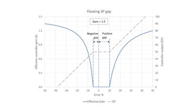
- Optimize tuning where the process normally runs and accept the possibility of instability if the process wanders into an area with a higher process gain. Adding a setpoint (SP) gap can stabilize the controller when the process wanders into high process gain areas, but at the expense of lower disturbance rejection in the normal operating area (see PID spotlight, part 32 for setup directions).
- Set stable tuning where the process has the highest gain and accept lower controller performance where the process normally runs.
- If possible, cascade a slow process to a flow controller. This often can linearize the slow controller by pushing the non-linearity into the flow controller. The fast response of the flow controller allows the use of “slow” tuning, which will still be much faster than the typical temperature or level controller, to avoid installing gain scheduling.
In refining, because most processes run within a narrow charge rate band, tuning is generally optimized for normal operations. On those rare occasions when the refinery is not in normal operations less than optimal tuning is accepted. Naturally, there are some processes that run through a wide range during normal operations, in which case controller gain scheduling will be used if necessary.
How to spot a non-linear process
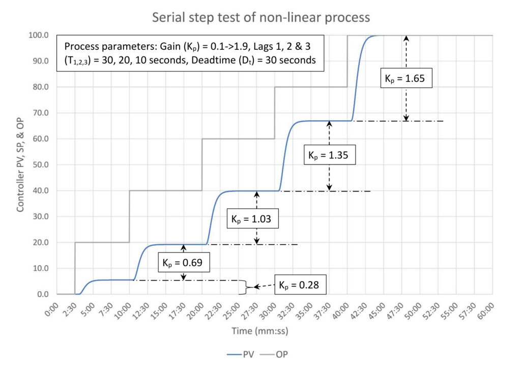
The easiest way to spot a non-linear process is to perform open loop step tests at multiple places, especially if the controller output steps could start at 0% and step through 100% as in Figure 1. But in an operating plant it would be unusual to be able to test at two places, much less over the full range. Regardless, Figure 1 highlights the nature of the problem; the calculated process gain depends on where the open loop step test starts. If the process never deviates from where the step test was performed then there will never be a controller performance problem (and no one will likely ever know there was a potential problem).
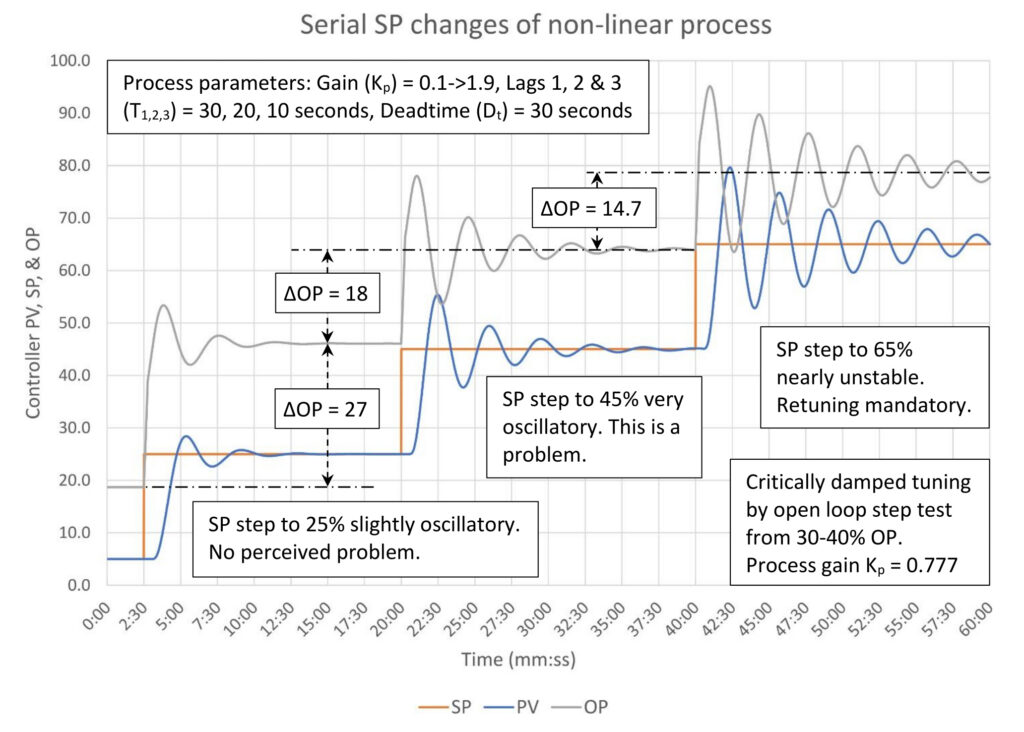
Figure 2: Critically damped PI tuning of a non-linear self-limiting process. Tuning constants are K = 0.873, Ti = 0.892 minutes/repeat, Td = 0 minutes. Courtesy: Ed Bullerdiek, retired control engineer
Most non-linear processes are discovered when a previously tuned controller starts to misbehave. Figure 2 is an example. The controller output (OP) was stepped between 30% and 40% during the open loop step test, resulting in an estimated process gain of 0.78. The controller is tuned for critically damped response. This is not very aggressive, yet by the time the setpoint (SP) is raised to 65%, the controller is nearly unstable. What often happens in this situation is the controller gets retuned and forgotten about. Ideally, the site maintains loop tuning logs, which should highlight that the controller gets tuned frequently. Further investigation should identify the non-linearity, which may lead to the installation of gain scheduling.
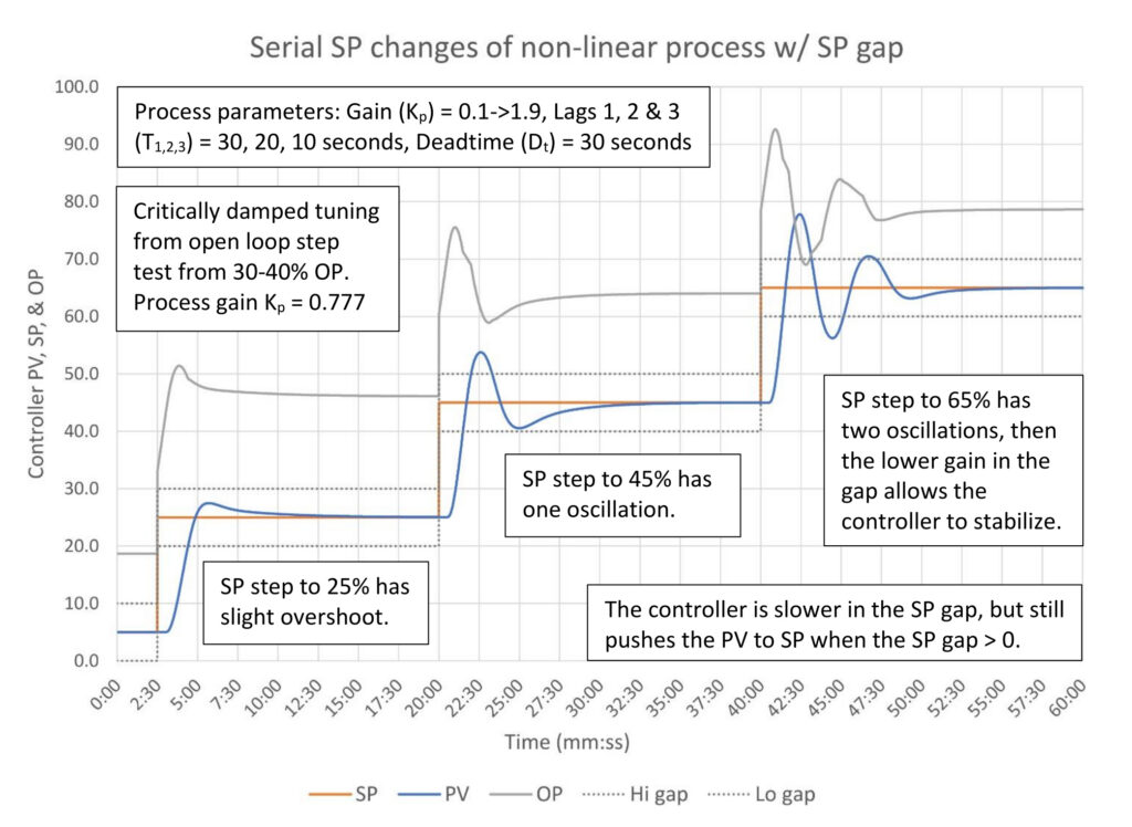
Figure 3: Critically damped PI tuning with SP notch gap of a non-linear self-limiting process. Tuning constants are K = 0.873, Ti = 0.892 minutes/repeat, Td = 0 minutes, SP gap limits ±5%, gap gain = 0.25. Courtesy: Ed Bullerdiek, retired control engineer
Before we dig into the process of setting up a gain scheduling application, in PID spotlight, part 32 we learned that an SP gap can stabilize otherwise unstable controller tuning. Figure 3 shows how adding an SP notch gap to the controller allows the controller to stabilize despite the high process gain. The controller gain gap factor is 0.25. This cuts the effective controller gain to 0.22, which is close to minimum OP movement tuning for the higher process gain when the process variable (PV) is at 65%. Because the SP gap gain is greater than zero, the PID controller still works, slowly, when the PV is inside the gap, and will always eliminate any error between the PV and SP.
Let’s note here that this could be considered a permanent solution, or a stopgap until a proper gain schedule can be developed. Nor would it be unusual to have to adjust the gap size and gap gain constant until a suitable tradeoff between performance and stability is found.
Does my control system support gain scheduling?
If your system does not support programmed modification of controller gain (integral and derivative) while the controller is in automatic or cascade mode, then controller gain scheduling is not possible.
If your system uses the parallel PID algorithm, then the gain scheduling program must also change integral (and derivative if used) proportionally to the changes in controller gain. This will add complexity to the calculations, but should work just as well.
If your system uses the positional form of the PID algorithm, then the gain schedule must be a smooth, continuous function to prevent sudden jumps in the controller output.
If you do not know these details about your system refer to PID spotlight, part 31 on how to test your system to determine the exact form of the PID algorithm.
What is the idea behind gain scheduling?
All open loop tuning methods calculate controller gain (K) by multiplying the inverse of the process gain (Kp) by some mathematical calculation (ƒ) involving the lag/deadtime ratio (T1/Dt).
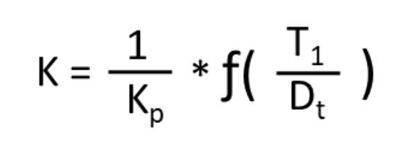
The PID controller assumes that the process gain, lag and deadtime do not change. Of course, in the real world, any or all of these can change as the process moves. For most processes, these don’t change enough to significantly affect controller operation, especially if the controller tuning is not aggressive.
The most common problem that requires gain scheduling is the process gain changes with the value of the process variable (PV). If this is all that changes, then calculating a moving controller gain can be reduced to:
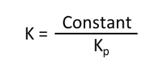
Then the only problem left is determining how the process gain Kp changes with the PV.
Before moving on, if the process lag or deadtime change based on any process parameter that can be measured, for example deadtime when transport delay changes with flow rate, then integral, derivative and even the controller gain can be recalculated using the appropriate open loop tuning calculations.
Methods to calculate process gain
While the math behind gain scheduling is conceptually easy, gathering the data usually is not. It is a tough ask to get operations management to support comprehensive testing across the full range of the controller. There are other methods to gather this data, each of which has a different difficulty level and accuracy. It is also not usually necessary to setup gain scheduling across the full range of the controller. Covering the normal operating range will usually be adequate, although some thought must be put into how to handle the high and low ends.
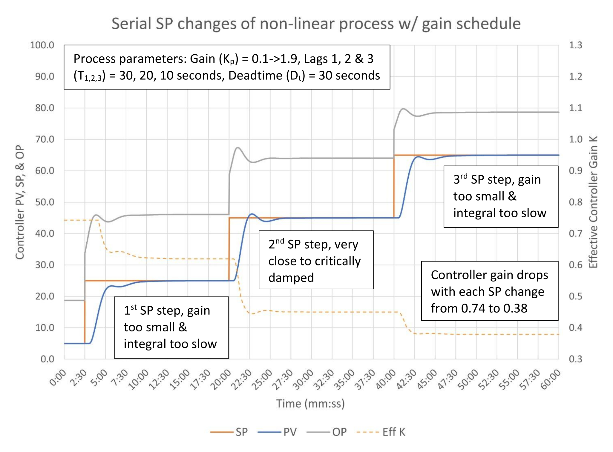
Figure 2 above shows us perhaps the easiest method to develop a partial gain schedule. Look through the trends for setpoint changes that cross different ranges. The process gain is the change in setpoint divided by the controller output movement. Assuming the control valve doesn’t stick a process gain can be calculated for each step. In this case for each 20% SP change the process gains are 0.74, 1.11 and 1.36 respectively. This data may not be terribly accurate, but it will get us started.
Other methods that can be used (in no particular order) include:
- A variation of looking through historical trends for SP changes is to do an X-Y plot of historical PV and OP data. A linear or quadratic regression can be used. Long-term instrument drift problems or frequent disturbances might affect the data. Shorter, carefully curated slices of data may yield better results. (Don’t dump a year of data in a spreadsheet and expect to get anything useful.)
- Formal open loop step tests across the controller span. This would be considered the gold standard because it will also tell you if the process deadtime or lag is changing with the PV. If this is significant then you can build schedules for controller gain, integral and, if used, derivative.
- If a dynamic simulator of reasonable accuracy is available, then you can step test the model. This eliminates having to work with operations, but, depending on the accuracy of the model, the tuning calculations could be inaccurate. At least one formal step test of the actual process will be required as a sanity check. (Dynamic models are very rare, but if one is available do not overlook the opportunity.)
- If a steady-state simulator is available, work with the process engineer to use the steady-state simulator to estimate process gains across the range of interest. This will not help with the process lag or deadtime. One open loop step test will be required to verify the data from the model represents the live process and to estimate lag and deadtime.
- This may be a long shot, but if the loop tuning logs either keep some data on the value of the PV at the time of the test or can be correlated with production campaigns, this may give you a start on setting up gain scheduling. This could be useful for batch and semi-batch manufacturers.
- Finally, gain schedules can be developed from engineering first principles and engineering documentation (such as pump/blower/compressor curves). This will likely be time consuming.
All of these methods to generate a process gain versus PV curve take time. When combined with the effort required for management of change, programming and documentation, we can easily understand why gain scheduling is often avoided. The reward must be worth the effort, which means this will usually be reserved for high impact, high value controllers.
Planning a gain scheduling implementation
Assuming you have the basic information to create a gain schedule, the next step is to perform an open loop step test (if test results aren’t already available). From this we will calculate the constant that will be divided by the process gain for the gain scheduling calculations. For demonstration purposes let’s use the critically damped controller gain calculation from PID spotlight, part 27, Table 2.
K = Kbase *(0.25 + 0.375 * T1/Dt)
The baseline controller gain (Kbase) is dropped from the calculation to yield:
Kconst = 0.25 + 0.375 * T1/Dt
From the step test the process lag (T1) is 0.827 minutes and the deadtime (Dt) is 0.723 minutes:
Kconst = 0.25 + 0.375 * 0.827/0.723
Kconst = 0.678
Any open loop tuning calculation set can be used. If your preference is lambda tuning (for example) the method remains the same.
Using the data from Figure 2, we have three calculated process gains, as the table shows:
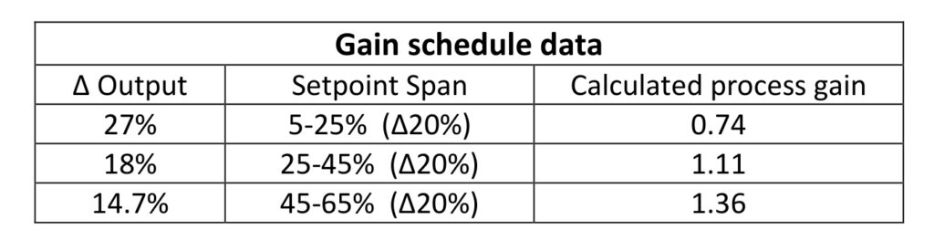
Table: Gain schedule test data for nonlinear process: Gain (Kp) = 0.1->1.9. Courtesy: Ed Bullerdiek, retired control engineer
There are some setup options to consider. One is whether the process gain is set at a fixed value within each setpoint span or should linear interpolation be used between the midpoint of each span? The second option is what happens when the process wanders outside those spans?
We can reasonably anticipate that the process gain changes continuously with the PV. We can see that the change in process gain is not linear. The large step sizes combined with the non-linearity of the rate of gain change suggests the calculated process gains aren’t that accurate. The best choice under the circumstances is to estimate the process gain using a linear interpolation between the midpoints of each step (15, 35, 55). Most systems supply a piecewise interpolation function, which makes this an easy choice.
Below 15% the actual process gain likely continues to drop, but the gain schedule process gain should not drop below 0.74 just in case this is a bad assumption. Above 55% the actual process gain likely still climbs. The safe option here is to continue raising the estimated process gain in a straight line. Based on this the estimated process gain when the PV is 100% is 1.9.
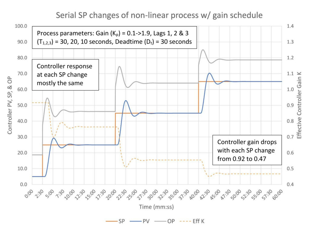
Figure 4: Critically damped PI tuning with gain scheduling of a non-linear self-limiting process. Tuning constants are Kconst = 0.678, Ti = 0.892 minutes/repeat, Td = 0 minutes. Courtesy: Ed Bullerdiek, retired control engineer
After the programming is completed the controller response to each setpoint change is substantially the same (Figure 4). The process variable overshoots the setpoint, so we didn’t exactly hit critically damped tuning, but the amount of overshoot is similar and the damping pattern of the following oscillations is identical. Over the course of the setpoint changes, the controller gain drops from 0.92 to 0.47, at each step following the shape of the PV. Given how we gathered the data to build the gain schedule this appears to be fairly successful.
From here heuristics say the integral is too fast (OP peak follows the PV peak) and controller gain is likely a little too high. Even though gain scheduling is installed, we can still use heuristic methods to trim up the controller response following the methods in PID spotlight, part 9. For this controller let’s slow down the integral about 25% to 1.1 minutes/repeat and lower the controller gain constant 20% to 0.55.
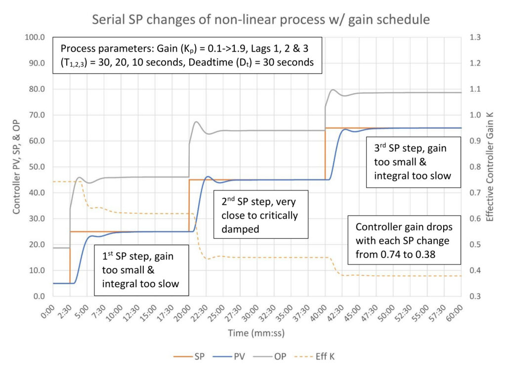
Figure 5: Critically damped PI tuning with gain scheduling of a non-linear self-limiting process. Tuning constants are Kconst = 0.55, Ti = 1.1 minutes/repeat, Td = 0 minutes. Courtesy: Ed Bullerdiek, retired control engineer
In Figure 5 it looks like the heuristic tuning adjustments went a little too far with both the controller gain and integral on the first and third setpoint step, but were reasonably close on step 2. This just tells us that our relatively quick gain schedule isn’t a perfect match to how the process is actually changing. This isn’t a surprise. In fact this is really quite good and compared to the controller response in Figure 2 this is a vast improvement.
To reemphasize the point of Figure 5, once a reasonable gain schedule is in place, you can use open loop and heuristic methods to retune a controller regardless of where the process is running at the time. The controller response should be substantially the same across the full range of the process provided the gain schedule reasonably follows the process. (Closed loop tuning cannot be used because it doesn’t yield an estimate of process lag or deadtime, which are required to calculate the constant (Kconst) required for the gain schedule calculation.)
What about gain scheduling with a positional PID controller?
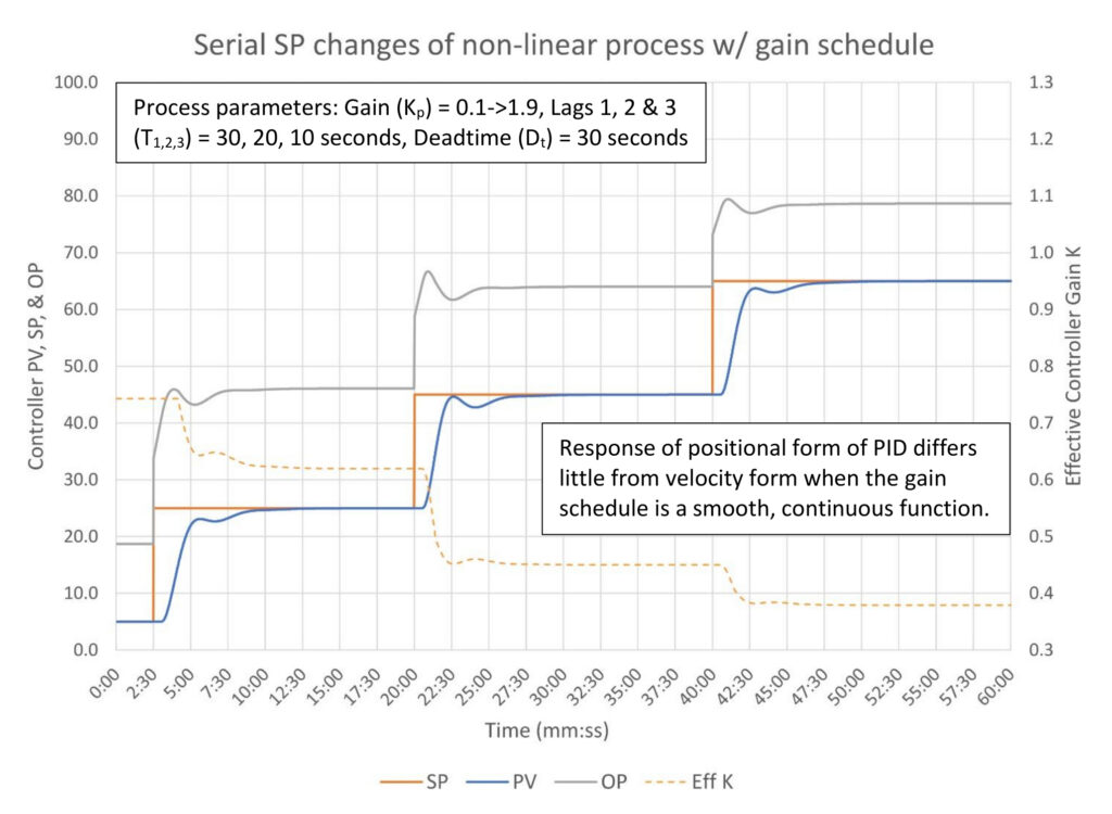
Figure 6: Critically damped PI tuning with gain scheduling of a non-linear self-limiting process. PID uses the positional form. Tuning constants are Kconst = 0.55, Ti = 1.1 minutes/repeat, Td = 0 minutes. Courtesy: Ed Bullerdiek, retired control engineer
Figure 6 is good news regarding gain scheduling with a positional PID algorithm. As long as the gain schedule is a smooth, continuous function the controller response will also be smooth. In fact, it should look very little different than the response of the velocity form PID algorithm in Figure 5. However, if there are discontinuities then, as we learned in PID spotlight, part 31, the controller output will jump. Note that you can accidently create a discontinuity if the gain schedule calculation is linked to the controller setpoint. The gain schedule calculation should be linked to the process variable. (But if it is linked to the setpoint, a short filter will suppress the sudden OP spikes when the SP is changed.)
Changing controller tuning when control objectives change
In PID spotlight, part 32, SP gap control was proposed for constraint control. This is predicated on the idea that the setpoint will be set up against the constraint and will never be changed; the controller’s specific purpose is to hold the process against the constraint. But there are controllers that do have constraints but are not specifically intended to hold the process against that constraint. These cases require custom gain scheduling rather than using the controller’s (usually) built in SP gap algorithm. The gain schedule will change at a fixed PV value (and the setpoint should be clamped inside the constraint limit.)
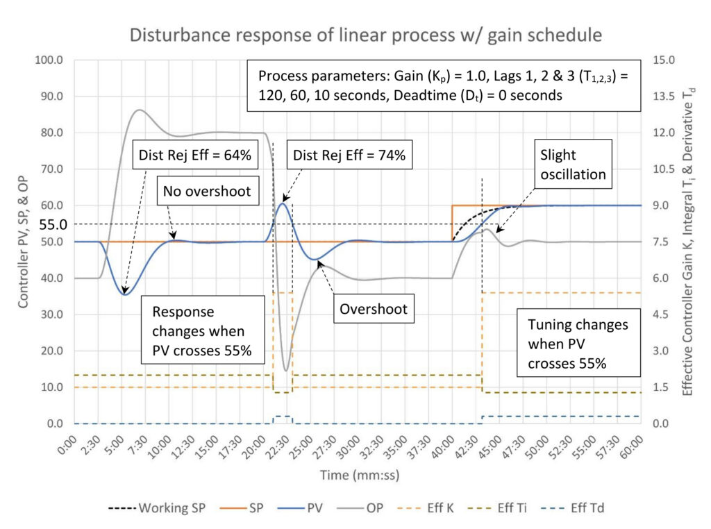
Figure 7: Gain scheduled PID tuning of a linear self-limiting process. Tuning constants: PV > 55; PID disturbance rejection: K = 5.4, Ti = 1.28 minutes/repeat, Td = 0.3 minutes. PV < 55; Critically damped: K = 1.5, Ti = 2.0 minutes/repeat, Td = 0 minutes. Courtesy: Ed Bullerdiek, retired control engineer
In Figure 7 the controller tuning is toggled between PID disturbance rejection and critically damped when the PV crosses 55%. The process has a 5.3:1 lag/deadtime ratio, therefore the disturbance rejection efficiency is very sensitive to controller tuning. This process is a good candidate for gain, integral and derivative scheduling.
A 40% disturbance in the safe direction occurs at the 2:30 minute-mark. Critically damped tuning corrects the disturbance without PV overshoot and a moderate amount of OP overshoot as expected. Disturbance rejection effectiveness is 64%, which is the expected performance for critically damped tuning for this process.
A 40% disturbance in the constrained direction occurs at the 20 minute-mark. Critically damped tuning is used until the PV crosses 55%, at which time PID disturbance rejection tuning is used. Despite the 5% delay, the disturbance rejection tuning improved the disturbance rejection effectiveness to 74%; less than the 80%+ possible, but noticeably more effective, nonetheless. The side effects of the more aggressive tuning include a large OP overshoot and the PV overshoots in the safe direction. These are expected impacts from the tuning change and are considered an acceptable tradeoff.
Finally, a setpoint change to 60% occurs at the 40 minute-mark. This should not be permitted, but has been included to show how the controller response changes when the PV does cross the 55% threshold to PID disturbance rejection tuning. Specifically, the controller output becomes oscillatory, warning us that stability may be a concern when very aggressive tuning is used above the constraint limit.
More gain scheduling with positional PID controllers
PID spotlight, part 31, included a discussion of how a sudden change in controller gain will result in a sudden jump in controller output if the control system uses the positional form of the PID algorithm. Figure 8 illustrates what this looks like with a real process.
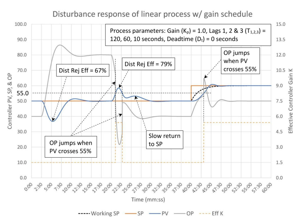
Figure 8: Gain scheduled PID tuning of a linear self-limiting process. Tuning constants: K = 1.5 when PV < 55%, 5.4 when PV > 55%, Ti = 1.65 minutes/repeat, Td = 0.3 minutes. Courtesy: Ed Bullerdiek, retired control engineer
The process and series of disturbances and setpoint changes in Figure 8 is identical to Figure 7. However, the PID algorithm is the positional form. In the interest of clarity the controller integral and derivative are constant throughout. They are instead set at blended values between PID disturbance rejection and critically damped. This is perfectly acceptable as long as the controller works well.
The controller response to the disturbance at the 2:30 minute-mark is little different. The disturbance rejection effectiveness is slightly better due to the integral being slightly faster and the presence of derivative. The tuning changes also result in the PV slightly overshooting the SP on the return.
The disturbance at the 20 minute-mark shows two sudden jumps in controller output. The first when the PV crosses above 55% is actually helpful because it accelerates the controller response to the disturbance, improving disturbance rejection effectiveness. However, when the PV drops below 55% the OP jumps up almost 20%, which considerably delays the final elimination of the disturbance. The tuning fix for this is to reduce the maximum gain, which will slow the initial response to the disturbance.
Finally the SP change at the 40 minute-mark results in a sudden 10% jump in the OP when the PV crosses 55%. This doesn’t disturb the process very much but is likely not good for other parts of the process.
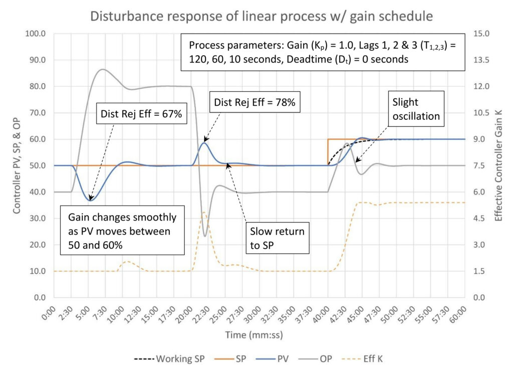
Figure 9: Gain scheduled PID tuning of a linear self-limiting process. Tuning constants: K = 1.5 when PV < 50%, 5.4 when PV > 60%, interpolated between, Ti = 1.65 minutes/repeat, Td = 0.3 minutes. Courtesy: Ed Bullerdiek, retired control engineer
Eliminating the sudden OP jumps requires converting the controller gain schedule to a continuous function. The easiest way to do this is to install a linear interpolation between two fixed values. This should be simple as most systems supply a piecewise linear interpolation function. In Figure 9 the controller gain is ramped using an interpolation function when the PV is between 50 and 60%. This achieves essentially identical controller performance to that seen in Figure 8 without the sudden OP jumps.
The disturbance at the 20 minute-mark resulted in slightly more PV movement from SP, but the return to setpoint, while still delayed, is much better than seen in Figure 8. Finally, the response to the SP change at the 40 minute-mark shows the slight OP oscillation we would expect from a very aggressively tuned controller.
The good news here is, if you should unknowingly stumble into a positional PID algorithm while using a stepped controller gain schedule, the problem can be easily fixed. In this case the step when the PV crosses 55% was changed to a ramp between 50 and 60%. The controller response remains nearly identical but without the sudden OP jumps.
Ed Bullerdiek is a retired control engineer with 37 years of process control experience in petroleum refining and oil production. Send comments and questions to [email protected]. Edited by Mark T. Hoske, editor-in-chief, Control Engineering, Arrowfly Media, [email protected].
Keywords
Proportional-integral-derivative, PID tutorial
Learning objectives
- Know when to consider controller gain scheduling and possible alternatives to gain scheduling.
- Know how to identify a non-linear process.
- Know how to plan for, identify and implement a gain schedule application.
- Understand that gain, integral and derivative scheduling can be used when control objectives change, for example for constraint control.
Consider this
If you have PID controllers that are detuned because the process is non-linear, controller gain scheduling can be used to improve control by matching controller response to the process no matter the process gain.
You also might like
PID series from Ed Bullerdiek, retired control engineer
PID Spotlight, part 1: Three reasons to tune control loops: Safety, profit, energy efficiency
PID spotlight, part 2: Know these 13 terms, interactions
PID spotlight, part 3: How to select one of four process responses
PID spotlight, part 4: How to balance PID control for a self-limiting process
PID spotlight, part 5: What does good and bad controller tuning look like?
PID spotlight, part 6: Deadtime? How to boost controller performance anyway
PID spotlight, part 7: Open-loop tuning of a self-limiting process
PID spotlight, part 8: Closed-loop tuning for self-limiting processes
PID spotlight, part 9: Heuristic tuning for a self-limiting process (part A on heuristic tuning)
PID spotlight, part 10: Heuristic tuning in a self-limiting process
PID spotlight, part 11: How a PID controller works with an integrating process
PID spotlight, part 12: What does good and bad controller tuning look like?
PID spotlight, part 13: Deadtime: what’s the best that I can do?
PID spotlight, part 14: Open loop tuning of an integrating process
PID spotlight, part 15: Open loop tuning of near integrating processes
PID spotlight, part 16: Closed loop tuning of an integrating process
PID spotlight, part 17: Heuristic tuning of an integrating processes
PID spotlight, part 18: Identifying control valve performance problems
PID spotlight, part 19: PID controller tuning mechanics
PID spotlight, part 20: Tuning with bad valves
PID spotlight, part 21: Noise: Can I tune around it?
PID spotlight, part 22: Can I tune a noisy PID controller?
PID spotlight, part 23: Filtering noise for better PID control
PID spotlight: part 24: How do I tune PID controllers during a new unit startup?
PID spotlight, part 25: Navigating PID controller tuning
PID spotlight, part 26: How fast should I tune my PID controller?
PID spotlight, part 27: Navigating PID controller tuning
PID spotlight, part 28: How well will my PID controller work?
PID spotlight, part 29: How to shape PID controller response – part 1
PID spotlight, part 30: How to shape PID controller response – integrating processes
PID spotlight, part 31: What is PID gap control?
PID spotlight, part 32: Shaping controller response using setpoint gap action
PID spotlight, part 33: Managing noise using setpoint gap action
More on PID and advanced process control from Control Engineering